Bayesian Theorem: Breaking it to Simple Using PyMC3 Modelling
Dr. Monika Singh
Consultant - Data Science & Analytics
Abstract
This article edition of Bayesian Analysis with Python introduced some basic concepts applied to the Bayesian Inference along with some practical implementations in Python using PyMC3, a state-of-the-art open-source probabilistic programming framework for exploratory analysis of the Bayesian models.
The main concepts of Bayesian statistics are covered using a practical and computational approach. The article covers the main concepts of Bayesian and Frequentist approaches, Naive Bayes algorithm and its assumptions, challenges of computational intractability in high dimensional data and approximation, sampling techniques to overcome challenges, etc. The results of Bayesian Linear Regressions are inferred and discussed for the brevity of concepts.
Introduction
Frequentist vs. Bayesian approaches for inferential statistics are interesting viewpoints worth exploring. Given the task at hand, it is always better to understand the applicability, advantages, and limitations of the available approaches.
In this article, we will be focusing on explaining the idea of Bayesian modeling and its difference from the frequentist counterpart. To make the discussion a little bit more intriguing and informative, these concepts are explained with a Bayesian Linear Regression (BLR) model and a Frequentist Linear Regression (LR) model.
Bayesian and Frequentist Approaches
The Bayesian Approach:
Bayesian approach is based on the idea that, given the data and a probabilistic model (which we assume can model the data well), we can find out the posterior distribution of the model’s parameters. For e.g.
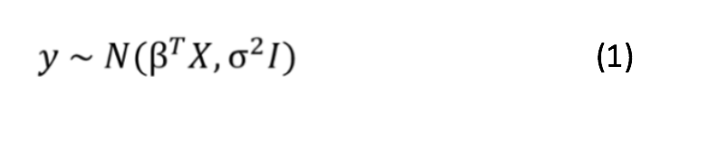
In Bayesian Linear Regression approach, not only the dependent variable y, but also the parameters(β) are assumed to be drawn from a probability distribution, such as Gaussian distribution with mean=βTX, and variance =σ2I (refer equation 1). The outputs of BLR is a distribution, which can be used for inferring new data points.
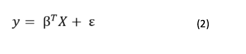
The Frequentist Approach, on the other hand, is based on the idea that given the data, the model and the model parameters, we can use this model to infer new data. This is commonly known as the Linear Regression Approach. In LR approach, the dependent variable (y) is a linear combination of weights term-times the independent variable (x), and e is the error term due to the random noise.
Ordinary Least Square (OLS) is the method of estimating the unknown parameters of LR model. In OLS method, the parameters which minimize the sum of squared errors of training data are chosen. The output of OLS are “single point” estimates for the best model parameter.
Let’s get started with Naive Bayes Algorithm, which is the backbone of Bayesian machine learning algorithms. Here, we can predict only one value of y, so basically it is a point estimation
Naive Bayes Algorithm for Classification
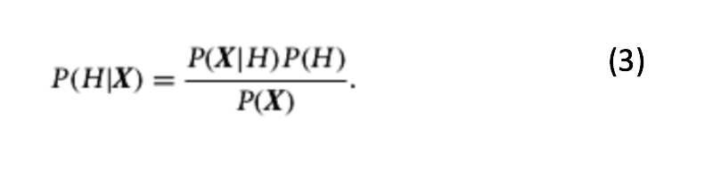
Discussions on Bayesian Machine Learning models require a thorough understanding of probability concepts and the Bayes Theorem. So, now we discuss Bayes’ Algorithm. Bayes’ theorem finds the probability of an event occurring, given the probability of an already occurred event. Suppose we have a dataset with 7 features/attributes/independent variables (x1, x2, x3,…, x7), we call this data tuple as X. Assume H is the hypothesis of the tuple belonging to class C. In Bayesian terminology, it is known as the evidence. y is the dependent variable/response variable (i.e., the class in classification problem). Then Mathematically, Bayes theorem is stated as :
Where:
P(H|X) is the probability that the hypothesis H holds correct, given that we know the ‘evidence’ or attribute description of X. P(H|X) is the probability of H conditioned on X, a.k.a., Posterior Probability.
P(X|H) is the posterior probability of X conditioned on H and is also known as ‘Likelihood’.
P(H) is the prior probability of H. This is the fraction of occurrences for each class out of total number of samples.
P(X) is the prior probability of evidence (data tuple X), described by measurements made on a set of attributes (x1, x2, x3,…, x7).
As we can see, the posterior probability of H conditioned on X is directly proportional to likelihood times prior probability of class and is inversely proportional to the ‘Evidence’.
Bayesian approach for regression problem:Assumptions of Bayes theorem, given a sales prediction problem with 7 independent variables.
i) Each pair of features in the dataset are independent of each other. For e.g., feature x1 has no effect on x2, & x2 has no effect on feature x7. ii) Each feature makes an equal contribution towards the dependent variable.
Finding the posterior distribution of model parameters is computationally intractable for continuous variables, we use Markov Chain Monte Carlo and Variational Inferencing methods to overcome this issue.
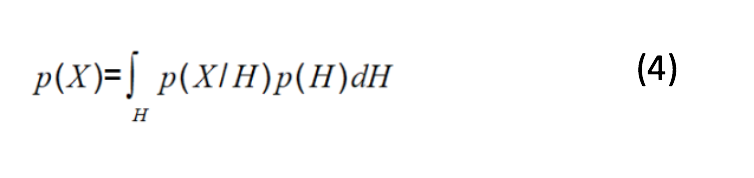
From Naive Bayes theorem (equation 3), posterior calculation needs a prior, a likelihood and evidence. Prior and likelihood are calculated easily as they are defined by the assumed model. As P(X) doesn’t depend on H and given the values of features, the denominator is constant. So, P(X) is just a normalization constant. We need to maximize the value of numerator in equation 3. However, the evidence (probability of data) is calculated as:
Calculating the integral is computationally intractable with high dimensional data. In order to build faster and scalable systems, we require some sampling or approximation techniques to calculate the posterior distribution of parameters given in the observed data. In this section, two important methods for approximating intractable computations are discussed. These are sampling-based approach. Markov-chain Monte Carlo Sampling (MCMC sampling) and approximation-based approach known as Variational Inferencing (VI). Brief introduction of these techniques are as mentioned below:
MCMC– We use sampling techniques like MCMC to draw samples from the distribution, followed by approximating the distribution of the posterior. Refer to George’s blog [1], for more details on MCMC initialization, sampling and trace diagnostics.
VI– Variational Inferencing method tries to find the best approximation of the distribution from a parameter family. It uses an optimization process over parameters to find the best approximation. In PyMC3, we can use Automatic Differentiation Variational Inference (ADVI), which tries to minimize the Kullback–Leibler (KL) divergence between a given parameter family distribution and the distribution proposed by the VI method.
Prior Selection: Where is the prior in data, from where do I get one?
Bayesian modelling gives alternatives to include prior information into the modelling process. If we have domain knowledge or an intelligent guess about the weight values of independent variables, we can make use of this prior information. This is unlike the frequentist approach, which assumes that the weight values of independent variables come from the data itself. According to Bayes theorem:
Now that the method for finding posterior distribution of model parameters are being discussed, the next obvious question based on equation 5 is how to find a good prior. Refer [2] for understanding how to select a good prior for the problem statement. Broadly speaking, the information contained in the prior has a direct impact on the posterior calculations. If we have a more “revealing prior” (a.k.a., a strong belief about the parameters), we need more data to “alter” this belief. The posterior is mostly driven by prior. Similarly, if we have an “vague prior” (a.k.a., no information about the distribution of parameters), the posterior is much driven by data. It means that if we have a lot of data, the likelihood will wash away the prior assumptions [3]. In BLR, the prior knowledge modelled by a probability distribution is updated with every new sample (which is modelled by some other probability distribution).
Modelling Using PyMC3 Library for Bayesian Inferencing
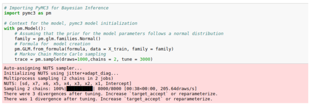
Following snippets of code (borrowed from [4]), shows Bayesian Linear model initialization using PyMC3 python package. PyMC3 model is initialized using “with pm.Model()” statement. The variables are assumed to follow a Gaussian distribution and Generalized Linear Models (GLMs) used for modelling. For an in-depth understanding on PyMc3 library, I recommend Davidson-Pilon’s book [5] on Bayesian methods.
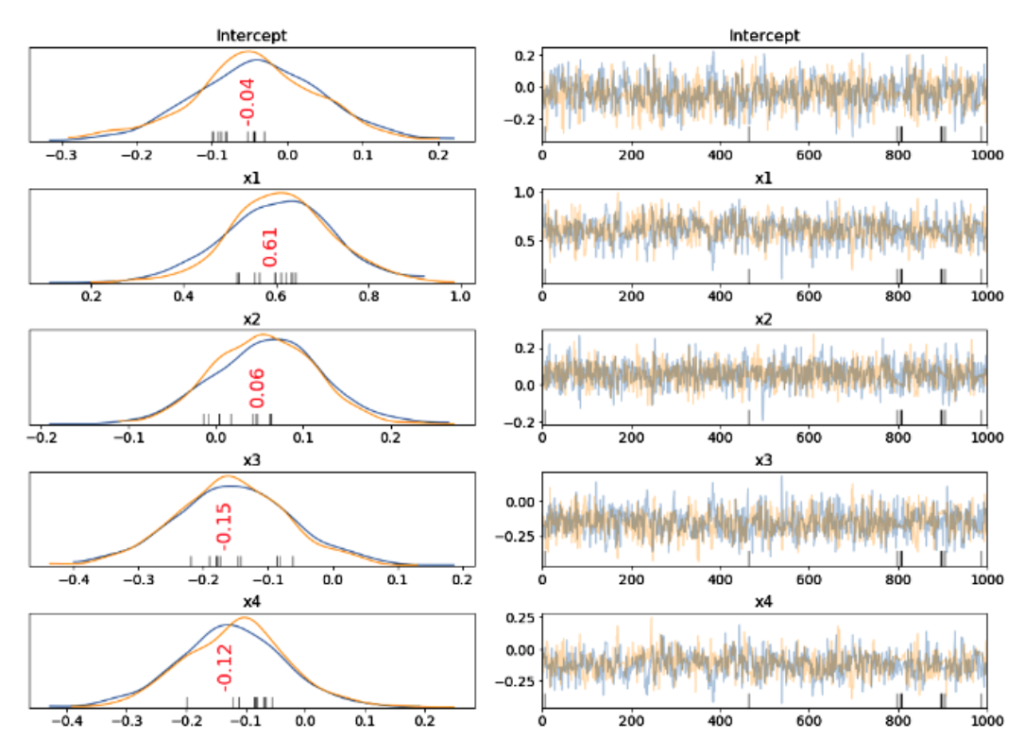
Fig. 1 Traceplot shows the posterior distribution for the model parameters as shown on the left hand side. The progression of the samples drawn in the trace for variables are shown on the right hand side.
We can use “Traceplot” to show the posterior distribution for the model parameters and shown on the left-hand side of Fig. 1. The samples drawn in the trace for the independent variables and the intercept for 1,000 iterations are shown on the right-hand side of the Fig 1. Two colours – orange and blue, represent the two Markov chains.
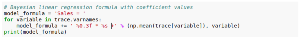
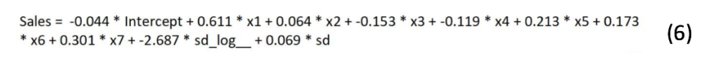
After convergence, we get the coefficients of each feature, which is its effectiveness in explaining the dependent variable. The values represented in red are the Maximum a posteriori estimate (MAP), which is the mean of the variable value from the distribution. The sales can be predicted using the formula:
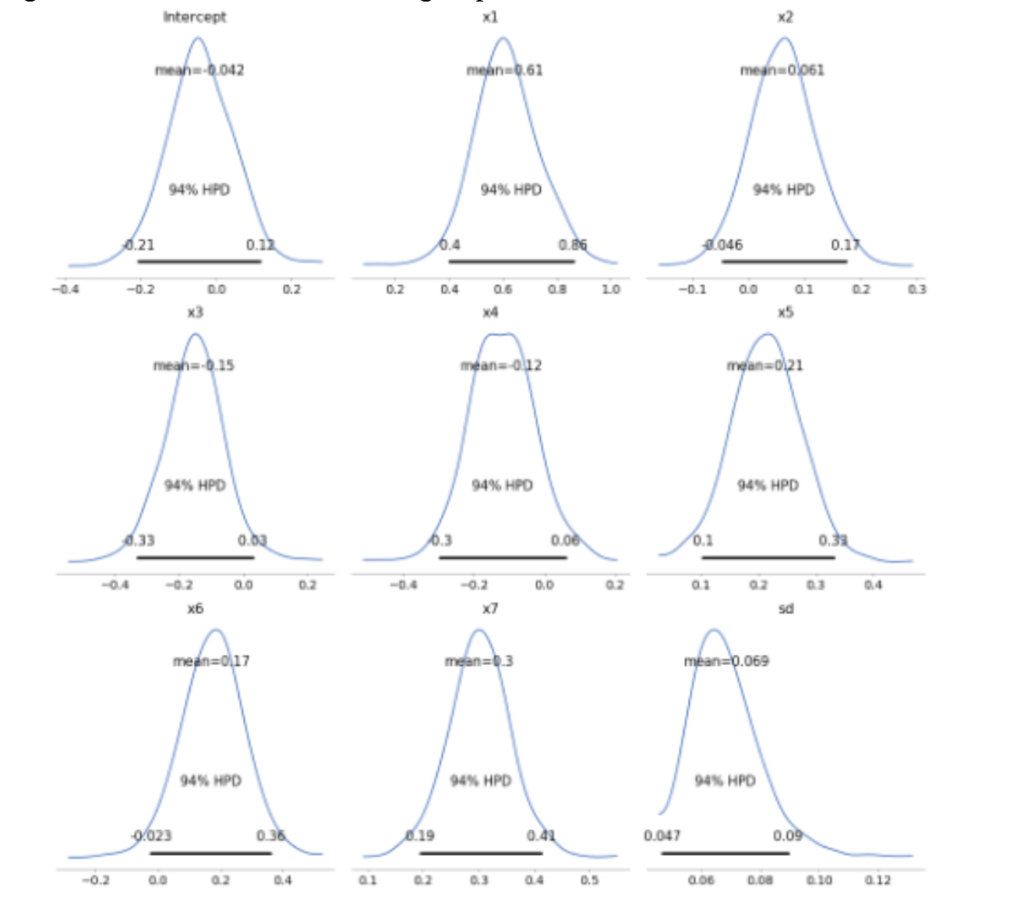
As it is a Bayesian approach, the model parameters are distributions. Following plots show the posterior distribution in the form of histogram. Here the variables show 94% HPD (Highest Posterior Density). HPD in Bayesian statistics is the credible interval, which tells us we are 94% sure that the parameter of interest falls in the given interval (for variable x6, the value range is -0.023 to 0.36).
We can see that the posteriors are spread out, which is an indicative of less data points used for modelling, and the range of values each independent variable can take is not modelled within a small range (uncertainty in parameter values are very high). For e.g., for variable x6, the value range is from -0.023 to 0.36, and the mean is 0.17. As we add more data, the Bayesian model can shrink this range to a smaller interval, resulting in more accurate values for weights parameters.
Fig. 2 Plots showing the posterior distribution in the form of histogram.
When to use linear and BLR, Map, etc. Do we go Bayesian or Frequentist?
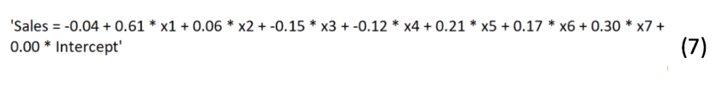
The equation for linear regression on the same dataset is obtained as:
If we see Linear regression equation (eq. 7) and Bayesian Linear regression equation (eq. 6), there is a slight change in the weight’s values. So, which approach should we take up? Bayesian or Frequentist, given that both are yielding approximately the same results?
When we have a prior belief about the distributions of the weight variables (without seeing the data) and want this information to be included into the modelling process, followed by automatic belief adaptation as we gather more data, Bayesian is a preferable approach. If we don’t want to include any prior belief and model adaptions, the weight variables as point estimates, go for Linear regression. Why are the results of both models approximately the same?
The maximum a posteriori estimates (MAP) for each variable is the peak value of the variable in the distribution (shown in Fig.2) close to the point estimates for variables in LR model. This is the theoretical explanation for real-world problems. Try using both approaches, as the performance can vary widely based on the number of data points, and data characteristics.
Conclusion
This blog is an attempt to discuss the concepts of Bayesian inferencing and its implementation using PyMC3. It started off with the decade’s old Frequentist-Bayesian perspective and moved on to the backbone of Bayesian modelling, which is Bayes theorem. Once setting the foundations, the concepts of intractability to evaluate posterior distributions of continuous variables along with the solutions via sampling methods viz., MCMC and VI are discussed. A strong connection between the posterior, prior and likelihood is discussed, taking into consideration the data available in hand. Next, the Bayesian linear regression modelling using PyMc3 is discussed, along with the interpretations of results and graphs. Lastly, we discussed why and when to use Bayesian linear regression.
Resources:
The following are the resources to get started with Bayesian inferencing using PyMC3.
Lorem Ipsum is simply dummy text of the printing and typesetting industry. Lorem Ipsum has been the industry's standard dummy text ever since the 1500s, when an unknown printer took a galley of type and scrambled it to make a type specimen book. It has survived not only five centuries, but also the leap into electronic typesetting, remaining essentially unchanged.