Back in 2014, Ian Goodfellow and his colleagues presented the much famous GANs(Generative Adversarial Networks) and it aimed at generating true to life images which were nearly unidentifiable to be outcome of a network.
Researchers found many use-cases where GANs could entirely change the future of ML industry but there were some shortcomings which had to be addressed. ProGAN and its successors improve upon the lacking areas and provide us with mind blowing results.
This post starts at understanding GAN basics and their pros and cons, then we dive into architectural changes incorporated into ProGAN, StyleGAN and StyleGAN2 in detail. It is assumed that you are familiar with concepts of CNN and overall basics of Deep neural nets.
Let’s Start-
Quick Recap into GANs —
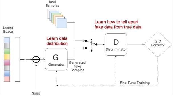
GANs are Generative model which aims to synthesize new data like training data such that it is becomes hard to recognize the real and fakes. The architecture comprises of two networks — Generator and Discriminator that compete against each other to generate new data instances.
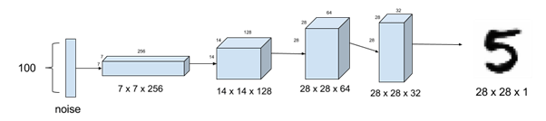
Generator: This network takes some random numbers/vector as an input and generates an image output. This output is termed as “fake” image since we will be learning the real image data distribution and attempt to generate a similar looking image.
Architecture: The network comprises of several transposed convolution layers aimed at up-scaling and turning the vector 1-D input to image. In below image we see that a 100-d input latent vector gets transformed into (28x28x1) image by successive convolution operations.
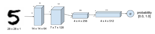
Discriminator: This network accepts generator output + real image(from training set) and classifies them as real or fake. In the below image, we see the generator output is fed into discriminator and then classified accordingly by a classifier network.
Both the networks are in continuous feedback, where the generator learns to create better “fakes” and discriminator learns to accurately classify “fakes” as “fake”. We have some predefined metrics to check generator performance but generally the quality of fakes tells the true story.
Overall GAN architecture and its training summary-
? Note: In the rest of the article Generator and Discriminator networks will be referred as G network and D network.
Here is the step-by-step process to understand the working of GAN model:
Create a huge corpus(>30k) of training data having clean object centric images and no sort of waste data. Once data gets created, we perform some more intermediate data prep steps(as specified in official StyleGAN repository) and start the training.
The G network takes a random vector and generates images, most of which will look like absolutely nothing or will be worse at start.
D network takes 2 inputs (fakes by G from step 1 + real images from training data) and classifies them as “real” or “fake”. Initially classifier will easily detect the fakes but once the training commences, G network will learn to fool the classifier.
After calculation of loss function, D network weights are being updated to make the classifier stricter. This making predicting fakes easy for D network.
Thereafter the G network updates its parameters and aims to improve the quality of images to match the training distribution with each iterative feedback from D network.
Important: Both the networks train in isolation, if the D network parameters get updated, G remain untouched and vice-versa.
This iterative training of G & D network continues till G produces good quality images and fools the D confidently. Thus both networks reach a stage known as “Nash equilibrium”.
? Limitations of GAN:
Mode collapse — The point at which generator produces same set of fakes over a period is termed as mode collapse.
Low-Res generator output— GANs work best when operated within low-res image boundaries(less than 100×100 pixels output) since generator fails to produce images with finer details which may yield high-res images. Thus high-res images can be easily classified as “fake” and thus discriminator network overpowers the generator network.
High volume of training data — Generation of fine results from generator requires lot of training data to be used because less the data more distinguishable the features will be from output fake images.
Let us start with knowing the basics of ProGAN architecture in next section and what makes it stand out.
Vanilla GAN and most of earlier works in this field faced the problem of low-resolution result images(‘fakes’). The architecture could perfectly generate 64- or 128-pixels square images but higher pixel images were difficult to handle (images above 512×512) by these models.
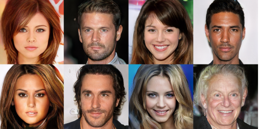
ProGAN (Progressive Growing GAN) is an extension to the GAN that allows generation of large high-quality images, such as realistic faces with the size 1024×1024 pixels by efficient training of generator model.
1.1 Understanding the concept :
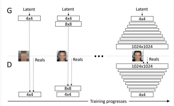
Progressive growing concept refers to changing the way generator and discriminator model architectures train and evolve.
Generator network starts with less Convolution layers to output low-res images(4×4) and then increments layers(to output high-res images 1024×1024) once the last smaller model converges. Similarly D network follows same approach, starts with smaller network taking the low-res images and outputs the probability. It then expands its network to intake the high-res images from generator and classify them as “real” or “fake”.
Both the networks expand simultaneously, if G outputs 4×4 pixel image then D network needs to have architecture that accepts these low-res image as shown below –
This incremental expansion of both G and D networks allows the models to effectively learn high level details first and later focus on understanding the fine features in high-res (1024×1024) pixel images. It also promotes model stability and lowering the probability of “mode collapse”.
We get an overview of how the ProGAN achieves generation of high-res images but for more detail into how the incremental transition in layers happens refer to the two best blogs —
ProGANs were the first iteration of GAN models that aimed at generating such high-res image output that gained much recognition. But the recent StyleGAN/StyleGAN2 has taken the level too high, so we will mostly focus on these two models in depth.
ProGAN expanded vanilla GANs capacity to generate high-res 1024-pixel square images but still lacked the control over the styling of the output images. Although its inherent progressive growing nature can be utilized to extract features from multiple scales in meaningful way and get drastically improved results but still lacked the fineness in output.
Facial features include high level features like face shape or body pose, finer features like wrinkles and color scheme of face and hair. All these features need to be learnt by model appropriately.
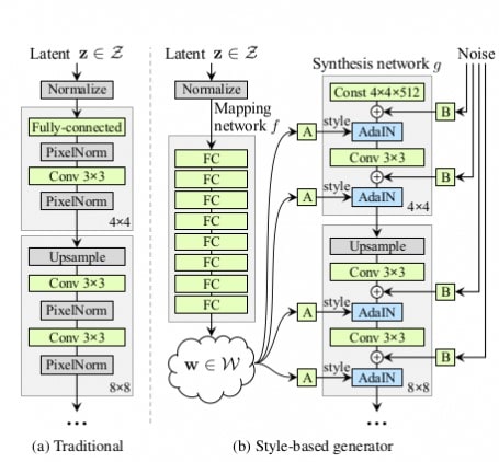
StyleGAN mainly improves upon the existing architecture of G network to achieve best results and keeps D network and loss functions untouched. Let us jump straight into the additional architectural changes –
Instead of directly injecting input random vector to G network, a standalone mapping network(f) is added that takes the same randomly sampled vector from the latent space(z) as input and generates a style vector(w). This new network comprises of 8 FC (fully connected)layers which outputs a 512-dimension latent vector similar in length to the input 512-d vector. Thus we have w = f(z) where both z,w are 512-d vectors. But a question remains.
What was the necessity to transform z w
“Feature entanglement” is the reason we need this transformation. In humans dataset, we see beard and short hair are associated with males which means these features are interlinked, but we need to remove that link (so we see guys have longer hair) for more diverse output and get control over what GANs can produce.
The necessity arises to disentangle features in the input random vector so as to allow a finer control on feature selection while generating fakes and the mapping network helps us achieve this mainly not following the training data distribution and reducing the correlation between features.
The G network in StyleGAN is renamed to “synthesis network” with the addition of the new mapping network to the architecture.
“You might be wondering? how this intermediate style vector adds into the G network layers”. AdaIN is the answer to that
2. AdaIN (Adaptive Instance Normalization):
To inject the styles into network layers, we apply a separately learned affine operation A to transform latent vector win each layer. This operation A generates a separate style y[ys, yb] (these both are scalars)from w whichis applied to each feature map when performing the AdaIN.
In the AdaIN operation, each feature map is normalized first and then scale(ys) + bias(yb) is applied to place the respective style information to feature maps.
Using normalization, we can inject style information into the G network in a much better way than just using an input latent vector.
The generator now has a sort of “description” of what kind of image it needs to construct (due to the mapping network), and it can also refer to this description whenever it wants (thanks to AdaIN).
3. Constant Input:
“Having a constant input vector ?”, you might be wondering why….?
Answer to this lies in AdaIN concept. Let us consider we are working on a vanilla GAN and off-course we require a different input random vector each time we want to generate a new fake with different styles. This means we are getting all different variations from input vector only once at start.
But StyleGAN has AdaIN & mapping network which allows to incorporate different styles/variations in input vector at every layer, then why we need a different input latent vector each time? Why can’t we work with constant input only?
G network no longer takes a point from the latent space as input but relies on a learned constant 4x4x512 value input to start the image synthesis process.
4. Adding Noise:
Need to have more fine-tuned output that looks more realistic? A small feature change can be added by the random noise being added to input vector which makes the fakes look truer.
A Gaussian noise (represented by B) is added to each of the activation maps before the AdaIN operations. A different sample of noise is generated for each block and is interpreted based on scaling factors of that layer.
5. Mixing regularization:
Using the intermediate vector at each level of synthesis network might cause network to learn correlation between different levels. This correlation needs to be removed and for this model randomly selects two input vectors (z1 and z2) and generates the intermediate vector (w1 and w2) for them. It then trains some of the levels with the first and switches (in a random split point) to the other to train the rest of the levels. This switch in random split points ensures that network do not learn correlation very much and produces different looking results.
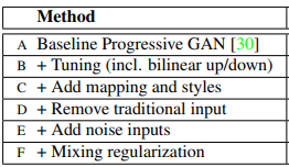
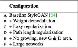
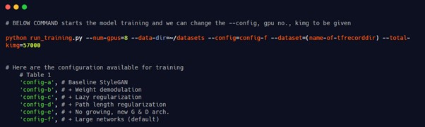
Training configurations: Below are different configurations for training StyleGAN which we discussed above. By default Config-F is used while training.
2.1. Let us have a look on Training StyleGAN on Custom dataset:
Pre-requisites– TensorFlow 1.10 or newer with GPU support, Keras version <=2.3.1. Other requirements are nominal and can be checked on official repository.
Below are the steps to be followed –
1. StyleGAN has been officially trained on FFHQ, LSUN, CelebHQ datasets which nearly contain more than 60k images. So looking at the count, our custom data must have around 30k images to begin with.
2. Images must square shaped(128,256,512,1024) and the size must be chosen to depend upon GPU or compute available for training model. 3. We will be using official repository for training steps. So let us clone the repository and start with next steps.
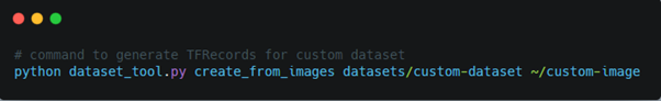
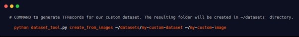
4. Data prep — Upload the image data folder to clone repository folder. Now we need to convert the images to TFRecords since the training and evaluation scripts only operate on TFRecord data, not on actual images. By default, the scripts expect to find the datasets at datasets/<NAME>/<NAME>-<RESOLUTION>.tfrecords
5. But why multi-resolution data Answer lies in the progressive growing nature of G and D network which train model progressively with increasing resolution of images. Below is script for generating TF-records for custom dataset –
Source for the custom source code format. Carbon.sh
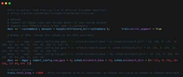
6. Configuring the train.py file: We need to configure the train file with our custom data TFRecord folder name present in datasets folder. Also there are some other main changes(shown in image below) related to kimgs and setting the GPUs available.
Train script from StyleGAN repo with additional parameter change comments
7. Start training — Run the train script withpython train.py. The model runs for several days depending on the training parameters given and images.
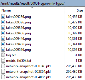
8. During the training, model saves intermediate fake results in the path results/<ID>-<DESCRIPTION>. Here we can find the .pkl model files which will be used for inference later. Below is a snap of my training progress.
Snapshot from self-trained model results
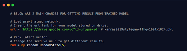
2.2. Inference using trained model: 1. Authors provide two scripts — pretrained_example.py and generate_figures.py to generate new fakes using our trained model. Upload your trained model to Google Drive and get corresponding model file link.
2. pretrained_example.py — Using this script we can generate fakes using different seed values. Changes required to file shown below –
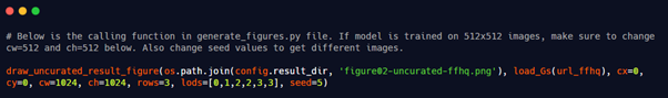
3. generate_figures.py — This script generates all sample images as shown in StyleGAN paper. Change the model url in the file and if you have used different resolution training images make changes as shown below. Suppose you trained model on 512×512 images.
2.3. Important mention:
Stylegan-encoder repository allows to implement style-mixing using some real-world test images rather than using seeds. Use the jupyter-notebook to implement some style-mixing and playing with latent directions.
StyleGAN surpassed the expectation of many researchers by creating astonishing high-quality images but after analyzing the results there were some issues found. Let us dive into the pain points first and then have a look into the changes made in StyleGAN 2.
Issues with StyleGAN-
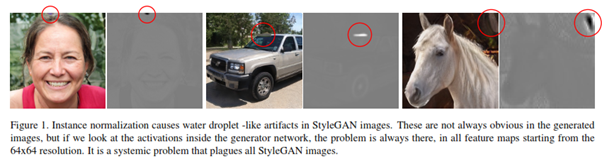
1. Blob(Droplet) like artifact: Resultant images had some unwanted noise which occurred in different locations. Upon research it was found that it occurs within synthesis network originating from 64×64 feature maps and finally propagating into output images.
This problem occurs due to the normalization layer (AdaIN). “When a feature map with a small spike-type distribution comes in, even if the original value is small, the value will be increased by normalization and will have a large influence”. Authors confirmed it by removing the normalization part and analyzing the results.
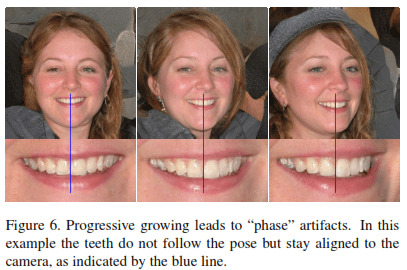
2. Phase artifacts: Progressive nature of GAN is the flag bearer for this issue. It seems that multiple outputs during the progressive nature causes high frequency feature maps to be generated in middle layers, compromising shift invariance.
StyleGAN2 like StyleGAN uses a normalization technique to infiltrate styles from W vector using learned transform A into the source imagebut now the droplet artifacts are being taken care of. They introduced Weight Demodulation for this purpose. Let us investigate changes made –
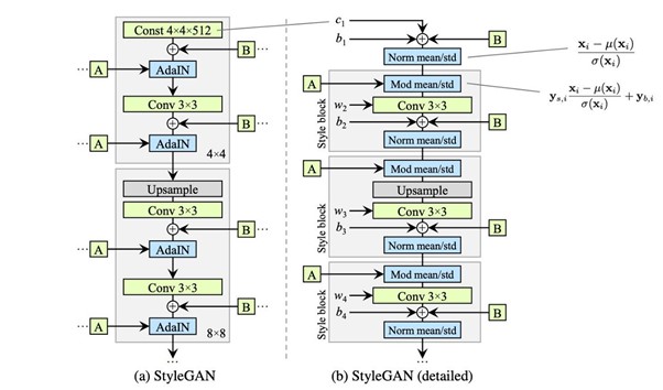
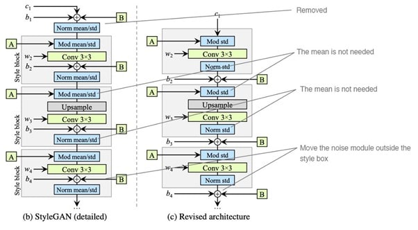
The first image(a) above shows the synthesis network from StyleGAN having 2 main inputs — Affine transformation (A) and input noise(B) applied to each layer. The next image(b) expands the AdaIN operation into respective normalization and modulation modules. Also each style(A) has been separated into different style blocks.
Let us discuss the changes in next iteration(image C)-
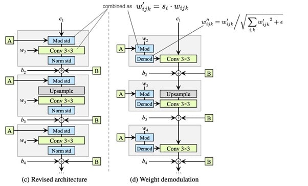
As seen in image above, we transform each style block by two operations-
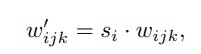
1. Combine modulation and convolution operation(Mod) by directly scaling the convolution weights rather than first applying modulation followed by convolution.
Source
Here w — original weight, w’ — modulated weight, si — scaling value for feature map i.
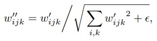
2. Next is the demodulation step(Demod), here we scale the output feature map j by standard deviation of output activations (from above step) and send to convolution operation.
Here small ε is added to avoid numerical operation issues. Thus entire style block in now integrated into single convolution layer whose weights are updated as described above. These changes improve training time, generate more finer results, and mainly remove blob like artifacts.
2 Lazy Regularization:
StyleGANs cost function include computing both main loss function + regularization for every mini-batch. This computation has heavy memory usage and computation cost which could be reduced by only computing
regularization term once after 16 mini-batches. This strategy had no drastic changes on model efficiency and thus was being implemented in StyleGAN2.
3 Path Length Regularization:
It is atype of regularization that allows good conditioning in the mapping from latent codes to images. The idea is to encourage that a fixed-size step in the latent space W results in a non-zero, fixed-magnitude change in the image. For a great detailed explanation please refer —
Progressive nature of StyleGAN has attributed to Phase artifacts wherein output images have strong location preference for facial features. StyleGAN2 tries to imbibe the capabilities of progressive growing(training stability for high-res images) and implements a new network design based on skip connection/residual nature like ResNet.
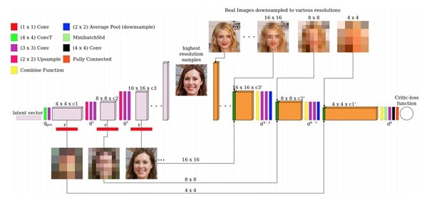
This new network does not expand to increase image resolution and yet produces the same results. This network is like the MSG-GAN which also uses multiple skip connections. “Multi-Scale Gradients for Generative Adversarial Networks” by Animesh Karnewar and Oliver Wang showcases an interesting way to utilize multiple scale generation with a single end-to-end architecture.
Below is actual architecture of MSG-GAN with the residual connections between G and D networks.
Source
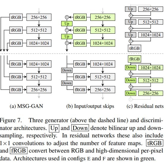
StyleGAN2 makes use of the different resolution features maps generated in the architecture and uses skip connections to connect low-res feature maps to final generated image. Bilinear Up/Down-sampling is used within the G and D networks.
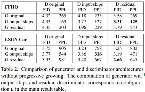
PPL values improves drastically in all combinations with G network having skip connections.
Residual D network and G output skip network give best FID and PPL values and is being mostly used. This combination of network is the configuration E for StyleGAN2.
5 Large Networks:
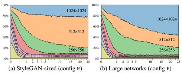
With all above model configurations explained, we now see the influence of high-res layers on the resultant image. The Configuration E yields the best results for both metrics as seen in last section. The below image displays contribution of different resolutions layers in training towards final output images.
The vertical axis shows the contribution of different resolution layers and horizontal axis depicts training progress. The best Config-E for StyleGAN2 has major contribution from 512 resolution layers and less from 1024 layers. The 1024 res-layers are mostly adding some finer details.
In general training flow, low-res layers dominate the output initially but eventually it is the final high-res layers that govern the final output. In Config-E, 512 res-layers seem to have more contribution and thus it impacts the output too. To get more finer results from the training, we need to increase the capacity of 1024 res-layers such that they contribute more to the output.
Config-F is considered a larger network that increases the feature maps in high-res layers and thus impacts the quality of resultant images.
3.3. Let us have a look on Training StyleGAN 2 on Custom dataset:
Pre-requisites– TensorFlow 1.14 or 1.15 with GPU support, Keras version <=2.3.1. Other requirements are nominal and can be checked on official repository.
Below are the steps to be followed – 1. Clone the repository — Stylegan2. Read the instructions in the readme file for verifying the initial setup on GPU and Tensorflow version.
2. Prepare the dataset(use only square shaped image with power of 2) as we did in StyleGAN training and place it in cloned folder. Now let us generate the multi-resolution TFRecords for our images. Below is the command –
3. Running training script: We do not need to change our training file, instead we can specify our parameters in the command only.
4. Like StyleGAN, here too our results will be stored into ./results/../ directory where we can see our model files(.pkl) and the intermediate fakes. Using the network-final.pkl file we will try generating some fakes with some random seeds as input.
3.4. Inference with random seeds:
Upload your trained model to Drive and get the download link to it.
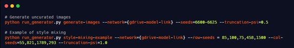
We will be using run_generator.py file for generating fakes and style-mixing results.
In the first command, we provide seeds from 6600–6625 which generates 25 fake samples from our model corresponding to each seed value. Thus we can change this range to get desired number of fakes.
Similarly for style-mix, there are row-seeds and col-seeds input which generate images for which we need to have style-mixing. Change the seeds and we will get different images each time.
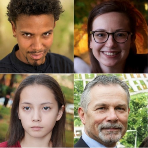
3.5 Results:
This sums up the StyleGAN2 discussion covering important architectural changes and training procedure. Below are the results generated and it gets rid of all issues faced by StyleGAN model.
Check out this great StyleGAN2 explanation by Henry AI Labs YouTube channel –
Thanks for going through the article. With my first article, I have attempted to cover an important topic in Vision area. If any error in the details is found, please feel free to highlight in comments.
References –
Custom code snippets: Create beautiful code snippets in different programming languages at https://carbon.now.sh/. All above snippets were created from the same website.
Lorem Ipsum is simply dummy text of the printing and typesetting industry. Lorem Ipsum has been the industry's standard dummy text ever since the 1500s, when an unknown printer took a galley of type and scrambled it to make a type specimen book. It has survived not only five centuries, but also the leap into electronic typesetting, remaining essentially unchanged.