Detectron2 FPN + PointRend Model for Amazing Satellite Image Segmentation

Satellite image segmentation has been in practice for the past few years, and it has a wide range of real-world applications like monitoring deforestation, urbanization, traffic, identification of natural resources, urban planning, etc. We all know that image segmentation is the process of color coding each pixel of the image into either one of the training classes. Satellite image segmentation is the same as image segmentation. In this process, we use landscape images taken from satellites and perform segmentation on them. Typical training classes include vegetation, land, buildings, roads, cars, water bodies, etc. Many Convolution Neural Network (CNN) models have shown decent accuracy in satellite image segmentation. One of these models, which is a highlight, is the U-Net model. Though the U-Net model gives decent accuracy, it still has some drawbacks like predicting classes with very near-distinguishable features, being unable to predict precise boundaries, and so on. In order to address these drawbacks, we have performed satellite image segmentation using the Basic FPN + PointRend model from the Detectron2 library, which has significantly rectified the drawbacks mentioned above and showed a 15% increase in accuracy when compared to the U-Net model on the validation dataset used.

In this blog, we will start by describing the objective of our experiment, the dataset we used, a clear explanation of the FPN + PointRend model architecture, and then demonstrate predictions from both U-Net and Detectron 2 models for comparison.

Objective

The main objective of this task is to perform semantic segmentation on satellite images to segment each image’s pixels into either of the five classes considered: greenery, soil, water, building, or utility. Constraints are anything related to plants and trees like forests, fields, bushes, etc., considered single-class greenery. Same for soil, water, building, and utility (roads, vehicles, parking lots, etc.) classes.

Data Preparation for Modeling

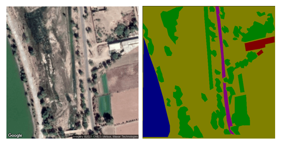
We have created 500 random RGB satellite images using the Google Maps API for modeling. For segmentation tasks, we need to prepare annotated images in the format of RGB masked images with height and width the same as the input image and each pixel value corresponds to the respective class color code (i.e., greenery – [0,255,0], soil – [255,255,0], water – [0,0,255], buildings – [255,0,0], utility – [255,0,255]). For the annotation process, we chose the LabelMe tool. Additionally, we have performed image augmentations like horizontal flip, random crop, and brightness alterations on images to let the model robustly learn the features. After annotations are done, we made a train and validation split for the dataset in the ratio of 90:10. Below is a sample image from the training dataset and the corresponding RGB masked image.

Model Understanding

For modeling, we have used the Basic FPN segmentation model + PointRend model from Facebook’s Detectron2 library. Now let us understand the architecture of both models.

Basic FPN Model

FPN (Feature Pyramid Network) mainly consists of two parts: encoder and decoder. An image is processed into a final output by passing through the encoder first, then through the decoder, and finally through a segmentation head for generating pixel-wise class probabilities. In the bottom-up encoder, the approach is performed using the ResNet encoder, and in the decoder, the top-down approach is performed using an adequately structured CNN network.

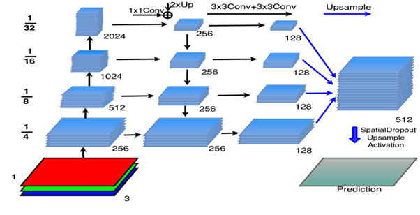
In the bottom-up approach, the RGB image is passed as input, and then it is processed through all the convolution layers. After passing through each layer, the output of that particular layer is sent as input to the next layer as well as input to the corresponding convolution layer in the top-down path, as seen in fig 2. In the bottom-up approach, image resolution is reduced by 1/4th the input resolution of that layer as we go up, therefore, performing down sampling on the input image.

In the top-down path for each layer, input comes from the above layer and from the corresponding bottom-up path layer, as seen in fig 2. These two inputs are merged and then sent to the layer for processing. Before merging to equate the channels of both input vectors, the input from the bottom-up path is passed through a 1*1 convolution layer, which results in an output of 256 channels, and the input from the above top-down layer is upsampled 2 times using the nearest neighbor’s interpolation method. Then both the vectors are added and sent as input to the top-down layer. The output of the top-down layer is passed 2 times successively through the 3*3 convolution layer, which results in a feature pyramid with 128 channels. This process is continued till the last layer in the top-down path. Therefore, the output of each layer in the top-down path is a feature pyramid.

Each feature map is upsampled such that its resulting resolution is the same as 1/4th of the input RGB image. Once upsampling is done, they are added and sent as input to the segmentation head, where 3*3 convolution, batch normalization, and ReLU activation are performed. To reduce the number of channels in the output to the same as the number of classes, we apply 1*1 convolution. Then spatial dropout and bi-linear interpolation upsampling are performed to get the prediction vector with the same resolution same as the input image.

Technically, in the FPN network, the segmentation predictions are performed on a feature map that has a resolution of 1/4th of the input image. Due to this, we must compromise on the accuracy of boundary predictions. To address this issue, PointRend model is used.

PointRend Model

The basic idea of the PointRend model is to see segmentation tasks as computer graphics rendering. Same as in rendering where pixels with high variance are refined by subdivision and adaptive sampling techniques, the PointRend model also considers the most uncertain pixels in semantic segmentation output, upsamples7t them, and makes point-wise predictions which result in more refined predictions. The PointRend model performs two main tasks to generate final predictions. These tasks are,

• Points Selection – how uncertain points are selected during inference and training
• Point-Wise Predictions – how predictions are made for these selected uncertain points

Points Selection Strategy

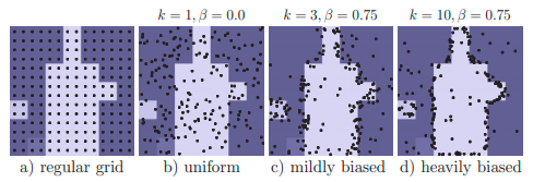
During inference, random points are selected where the probabilities in the coarse prediction output (prediction vector which has a resolution equal to 1/4th of the input image) from the FPN model have class probabilities near to 1/no. of the classes, i.e., 0.2 in our case as we have 5 classes. But during training, instead of selecting points only based on probabilities first, it selects kN random points from a uniform distribution. Then it selects βN most uncertain points (points with low probabilities) from among these kN points. Finally, the remaining (1 – β)N are sampled from a uniform distribution. For the segmentation task during training, k=3 and β=0.75 have shown good results. See fig 3 for more details on the point selection strategy during training.

Point-Wise Predictions

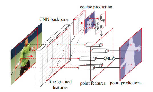
Point-wise predictions are made by combining two feature vectors:

• Fine-Grained Features – At each selected point, a feature vector is extracted from the CNN feature maps. The feature vector can be extracted from a single feature map of res2 or multiple feature maps, e.g., res2 to res5 or feature pyramids.
• Coarse Prediction Features – Feature maps are usually generated at low resolutions. Due to this fine feature, information is lost. For this, instead of relying completely on feature maps, course prediction output from FPN is also used in the extracted feature vector at selected points.

The combined feature vector is passed through MLP (multi-layer perceptron) head to get predictions. The MLP has a weight vector for each point, and these get updated during training by calculating loss similar to the FPN model, which is categorical cross-entropy.

Combined Model (FPN + PointRend) Flow

Now that we understand the main tasks of the PointRend model, let’s understand the flow of the complete task.

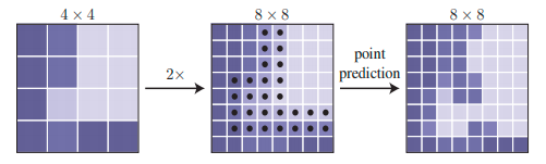
First, the input image is sent to the CNN network (in our case, the FPN model) to get a coarse prediction output (in our case, a vector of ¼th the resolution of the input image with 5 channels). This coarse prediction vector is sent as input to the PointRend model, where it is upsampled 2* times using bilinear interpolation, and N uncertain points are generated using the PointRend point selection strategy. Then, at these points, new predictions are made using a point-wise prediction strategy with a MLP head (multi-layer perceptron), and this process is continued till we reach the desired output resolution. Suppose the course prediction output resolution is 7*7 and the desired output resolution is 224*224; the PointRend upsampling is done 5 times. In our case, the input resolution is ¼th of the desired output resolution. Therefore, PointRend upsampling is performed twice. Refer to fig. 4 and 5 for a better understanding of the flow.

Results

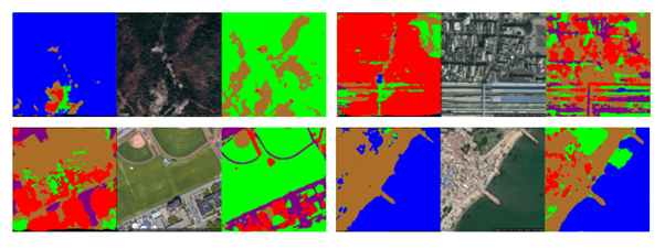
For model training, we have used Facebook’s Detectron2 library. The training was done using an Nvidia Titan XP GPU with 12GB of VRAM and performed for 1 lakh steps with an initial learning rate of 0.00025. The best validation IoU was obtained at the 30000th step. The accuracy of Detectron2 FPN + PointRend outperformed the UNet model for all classes. Below are some of the predictions from both models. As you can see Detectron2 model was able to distinguish features of greenery and water class when U-Net failed in almost all cases. Even the boundary predictions of the Detectron2 model are far better than U-Net’s.

Takeaway

In this blog, we have understood how the Detectron 2 FPN + PointRend model performs segmentation on the input image. The PointRend model can be applied as an extension to any image segmentation tasks to get better predictions at class boundaries. As further steps to improve accuracy, we can increase the training dataset, do augmentations on images, and play with hyperparameters like learning rate, decay, thresholds, etc.

Reference

[1] Feature Pyramid Network for Multi-Class Land Segmentation

[2] PointRend: Image Segmentation as Rendering