Explainable AI

The advancement in AI technology has led us to solve several problems with technology working side by side. The complexity of these AI models is growing, and so is the need to understand them. A growing concern is to regulate the bias in AI, which can occur for several reasons. One of many reasons is partial input data that will cause bias in the training model. So, it becomes increasingly essential to comprehend how the algorithm came to a result. Explainable AI is a set of tools and frameworks to help you understand and interpret predictions made by your machine learning models.
“Explainable artificial intelligence (XAI) is a set of processes and methods that allows human users to comprehend and trust the results and output created by machine learning algorithms. Explainable AI is used to describe an AI model, its expected impact, and potential biases.” -IBM
Feature Attributions
Feature attributions depict how much each feature in your model contributed to each instance of test data’s predictions. When you run explainable AI techniques, you get the predictions and feature attribution information.
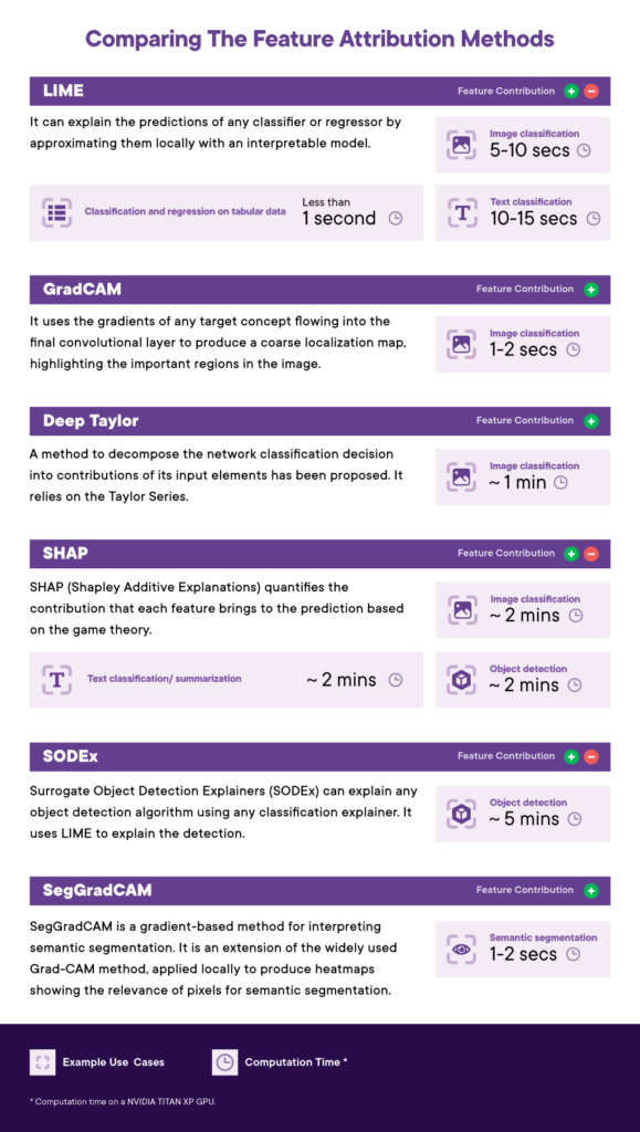
Understanding the Feature Attribution Methods
LIME
LIME is termed “Local Interpretable Model Agnostic Explanation.” It explains any model by approximating it locally with an interpretable model. It first creates a sample dataset locally by permuting the features or values from the original test instance. Then, a linear model is fitted to the perturbed dataset to understand the contribution of each feature. The linear model gives the final weight of each feature after fitting, which is the LIME value of these features. LIME has several methods based on the different models’ architecture and the input data.
LIME provides a tabular explainer that explains predictions based on tabular data. We implemented LIME for classification on the Iris dataset and regression on the Boston housing dataset. In the image below, we can see that petal length contributes positively to the Setosa class, whereas sepal length negatively contributes. Similarly, LSTAT and RM are the most contributing features in predicting Boston house prices.
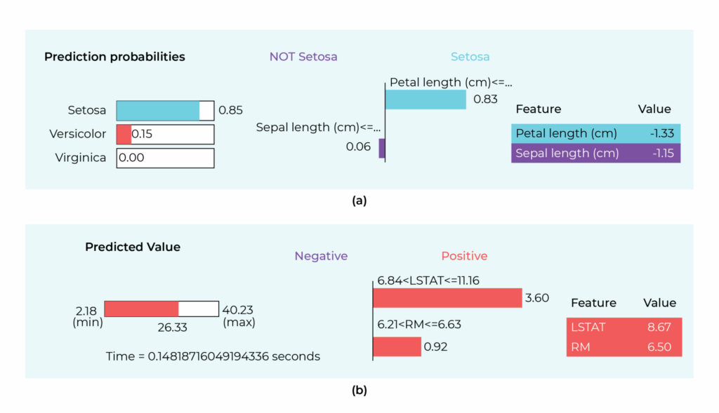
(b) LIME explanation for linear regression trained on Boston housing dataset.
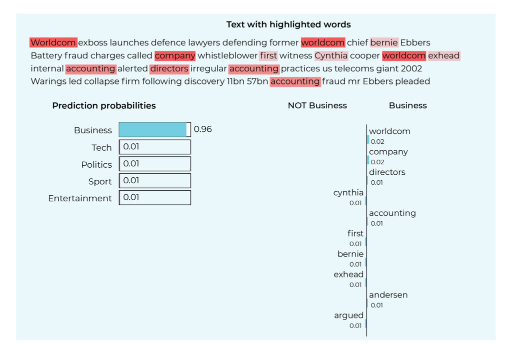
The sample dataset is created in text data by randomly permuting the words from the original text instance. The relevance of terms contributing to the prediction result is determined by fitting a linear model on the sample dataset.
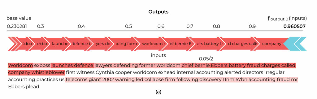
In the following text classification example, LIME highlights both positively and negatively contributing words towards the classification of the text in business class. The term “WorldCom” is contributing the most positively.
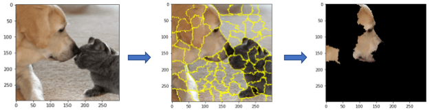
For image classification tasks, LIME finds the region of an image (set of super-pixels) with the strongest association with a prediction label. It generates perturbations by turning on/off some of the super-pixels in the image. Then a model to be explained predicts the target class on perturbated image. Next, a linear model is trained using the dataset of “perturbed” samples with their responses, which provides the weightage of super pixels.
In the example below LIME show the area which have strong association with the prediction of “Labrador”.
GradCAM
GradCAM stands for Gradient-weighted Class Activation Mapping. It uses the gradients of any target concept (say, “dog” in a classification network) flowing into the final convolutional layer. It works by evaluating the predicted class’s score gradients concerning the convolutional layer’s feature maps, which are then pooled to determine the weighted combination of feature maps. These weights are passed through the ReLu activation function to get the positive activations, producing a coarse localization map highlighting the critical regions in the image for predicting the concept.
We implement GradCAM to understand a CNN model trained on a human activity recognition dataset. In the following image, the most positive contributing area to the predicted class is shown in red, whereas the area in blue has no positive contribution towards the predicted class.

Deep Taylor
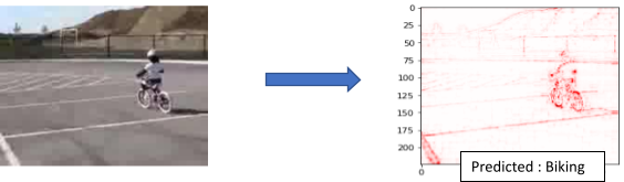
It is a method to decompose the output of the network classification into the contributions (relevance) of its input elements using Taylor’s theorem, which gives an approximation of a differentiable function. The output neuron is first decomposed into input neurons in a neural network. Then, the decomposition of these neurons is redistributed to their inputs, and the redistribution process is repeated until the input variables are reached. Thus, we get the relevance of input variables in the classification output.
As we can see in the image below, the pixels of the bicycle have the maximum contribution in the predicted biking class.
SHAP
Shapley values are a concept in a cooperative game theory algorithm that assigns credit to each player in a game for a particular outcome. When applied to machine learning models, this indicates that each model feature is considered as a “player” in the game, with AI Explanations allocating each proportionate feature credit for the prediction’s result. SHAP provides various methods based on model architecture to calculate Shapley values for different models.
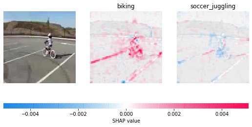
The SHAP gradient explainer is a method to drive the SHAP value on the image data. It calculates the gradient of the output score with respect to the input, i.e., the pixel’s intensity—this feature attribution method is designed for differentiable models like convolutional neural networks.
In the following image, the pixels in red are most positively contributing to the biking class. In contrast, the pixels in blue are confusing the model with a different class and hence negatively contributing.
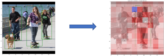
The SHAP kernel explainer is the only method that is model agnostic for the calculation of Shapley values. It is an extended and adapted method of linear LIME to calculate Shapley values. The Kernel Explainer builds a weighted linear regression using your data and predictions. Whatever function indicates the predicted values, the coefficients of the solution of weighted linear regression are the Shapley values. As a result, a gradient-based explanation method cannot be used since object detection models are non-differentiable. However, we can use the SHAP kernel explainer.
This method explains one detection in one image. Here we are explaining the person in the middle. We see that the dark red patches with the highest contribution are located within the bounding box of our target. Interestingly, the highest contribution seems to come from head and shoulders.
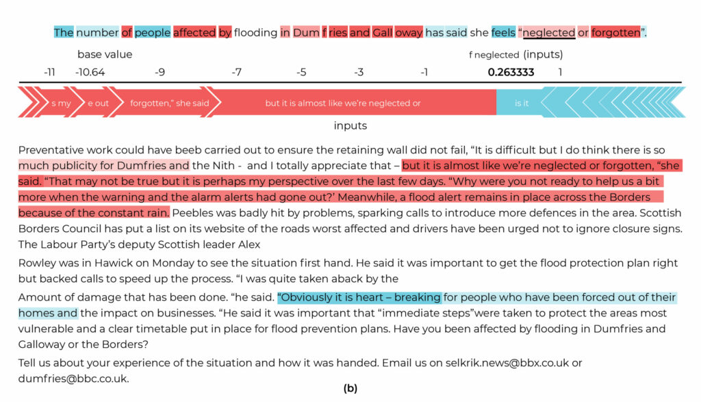
SHAP also has the functionality to derive explanations for NLP models. We demonstrate the use of SHAP for text classification and text summarization, which explains the contribution of words or a combination of words towards a prediction.
As we can see below, for example, in the text classification, the word “company” is the highest contributor in classifying text into the business class. In summary, the term “neglected” has “but it is almost like we are neglected” as its highest contributor in the text summarization.
SODEx
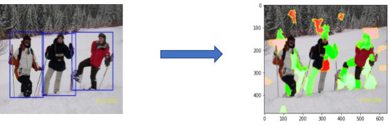
The Surrogate Object Detection Explainer (SODEx) explains an object detection model using LIME, which explains a single prediction with a linear surrogate model. It first segments the image into super pixels and generates perturbed samples. Then, the black box model predicts the result of every perturbed observation. Using the dataset of perturbed samples and their responses, it trains a surrogate linear model that provides super pixel weights.
It gives explanations for all the detected objects in an image. The green-colored patches show positive contributions, and the red-colored patches negatively contribute. Here, the model focuses on hands and legs to detect a person.
SegGradCAM
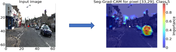
SEG-GRAD-CAM is an extension of Grad-CAM for semantic segmentation. It can generate heat maps to explain the relevance of the decisions of individual pixels or regions in the input image. The GradCAM uses the gradient of the logit for the predicted class with respect to chosen feature layers to determine their general relevance. But a CNN for semantic segmentation produces logits for every pixel and class. This idea allows us to adapt GradCAM to a semantic segmentation network flexibly since we can determine the gradient of the logit of just a single pixel, or pixels of an object instance, or simply all pixels of the image.
Like in GradCAM, the red pixels are the most positively contributing, whereas the pixels in blue have zero positive contributions. Here, the pixels of the car’s windscreen have the maximum contribution.
Conclusion
Explainable AI builds confidence in the model’s behavior by ensuring that the model does not focus on idiosyncratic details of the training data that will not generalize to unseen data. Therefore, it guarantees the fairness of ML models. We have implemented the explainable AI techniques for the models trained on tabular, text, and image data, thus enhancing these models’ transparency and interactivity. You can then use this information to verify that the model is behaving as expected, recognize bias in your models, and get ideas for improving your model and training data.
References
- Selvaraju et al. “Grad-CAM: Visual Explanations from Deep Networks via Gradient-based Localization.” International Journal of Computer Vision 2019
- http://www.heatmapping.org/slides/2018_ICIP_2.pdf
- https://towardsdatascience.com/shap-shapley-additive-explanations-5a2a271ed9c3
- Sejr, J.H.; Schneider-Kamp, P.; Ayoub, N. Surrogate Object Detection Explainer (SODEx) with YOLOv4 and LIME
- https://www.steadforce.com/blog/explainable-object-detection
- Vinogradova, K., Dibrov, A., & Myers, G. (2020). Towards Interpretable Semantic Segmentation via Gradient-Weighted Class Activation Mapping