Gradient Boosting Trees for Classification: A Beginner’s Guide

Introduction
Machine learning algorithms require more than just fitting models and making predictions to improve accuracy. Nowadays, most winning models in the industry or in competitions have been using Ensemble Techniques to perform better. One such technique is Gradient Boosting.
This article will mainly focus on understanding how Gradient Boosting Trees works for classification problems. We will also discuss about some important parameters, advantages and disadvantages associated with this method. Before that, let us get a brief overview of Ensemble methods.
What are Ensemble Techniques ?
Bias and Variance — While building any model, our objective is to optimize both variance and bias but in the real-world scenario, one comes at the cost of the other. It is important to understand the trade-off and figure out what suits our use case.
Ensembles are built on the idea that a collection of weak predictors, when combined, give a final prediction which performs much better than the individual ones. Ensembles can be of two types —
i) Bagging — Bootstrap Aggregation or Bagging is a ML algorithm in which a number of independent predictors are built by taking samples with replacement. The individual outcomes are then combined by average (Regression) or majority voting (Classification) to derive the final prediction. A widely used algorithm in this space is Random Forest.
ii) Boosting — Boosting is a ML algorithm in which the weak learners are converted into strong learners. Weak learners are classifiers which always perform slightly better than chance irrespective of the distribution over the training data. In Boosting, the predictions are sequential wherein each subsequent predictor learns from the errors of the previous predictors. Gradient Boosting Trees (GBT) is a commonly used method in this category.
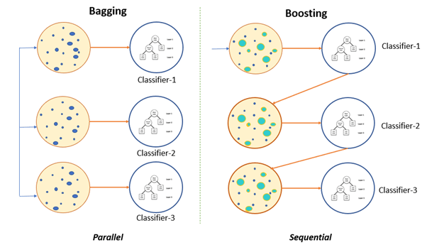
Fig 1. Bagging (independent predictors) vs. Boosting (sequential predictors)
Performance comparison of these two methods in reducing Bias and Variance — Bagging has many uncorrelated trees in the final model which helps in reducing variance. Boosting will reduce variance in the process of building sequential trees. At the same time, its focus remains on bridging the gap between the actual and predicted values by reducing residuals, hence it also reduces bias.
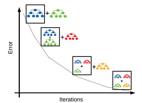
Fig 2. Gradient Boosting Algorithm
What is Gradient Boosting ?
It is a technique of producing an additive predictive model by combining various weak predictors, typically Decision Trees.
Gradient Boosting Trees can be used for both regression and classification. Here, we will use a binary outcome model to understand the working of GBT.
Classification using Gradient Boosting Trees
Suppose we want to predict whether a person has a Heart Disease based on Chest Pain, Good Blood Circulation and Blocked Arteries. Here is our sample dataset —
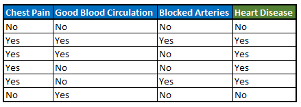
Fig 3: Sample Dataset
I. Initial Prediction — We start with a leaf which represents an initial prediction for every individual. For classification, this will be equal to log(odds) of the dependent variable. Since there are 4 people with and 2 without heart disease, log(odds) is equal to –
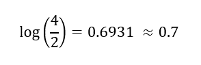
Next, we convert this to a probability using the Logistic Function –
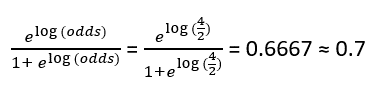
If we consider the probability threshold as 0.5, this means that our initial prediction is that all the individuals have Heart Disease, which is not the actual case.
II. Calculate Residuals — We will now calculate the residuals for each observation by using the following formula,
Residual = Actual value — Predicted value
where Actual value= 1 if the person has Heart Disease and 0 if not and Predicted value = 0.7
The final table after calculating the residuals is the following —
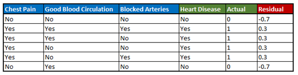
Fig 4. Sample dataset with calculated residuals
III. Predict residuals — Our next step involves building a Decision Tree to predict the residuals using Chest Pain, Good Blood Circulation and Blocked Arteries.
Here is a sample tree constructed —
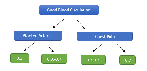
Fig 5. Decision Tree — While constructing the tree, its maximum depth has been limited to 2
Since the number of residuals is more than the number of leaves, we can see that some residuals have ended up in the same leaf.
How do we calculate the predicted residuals in each leaf?
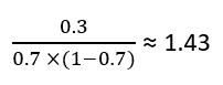
The initial prediction was in terms of log(odds) and the leaves are derived from a probability. Hence, we need to do some transformation to get the predicted residuals in terms of log(odds). The most common transformation is done using the following formula —
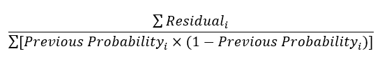
Applying this formula to the first leaf, we get predicted residual as –
Similarly, we calculate the predicted residuals for the other leaves and the decision tree will finally look like —
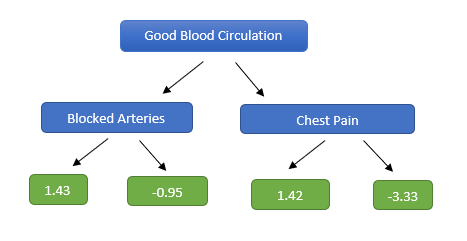
Fig 6. Modified Decision Tree
IV. Obtain new probability of having a heart disease — Now, let us pass each sample in our dataset through the nodes of the newly formed decision tree. The predicted residuals obtained for each observation will be added to the previous prediction to obtain whether the person has a heart disease or not.
In this context, we introduce a hyperparameter called the Learning Rate. The predicted residual will be multiplied by this learning rate and then added to the previous prediction.
Why do we need this learning rate?
It prevents overfitting. Introducing the learning rate requires building more Decision Trees, hence, taking smaller steps towards the final solution. These small incremental steps help us achieve a comparable bias with a lower overall variance.
Calculating the new probability –
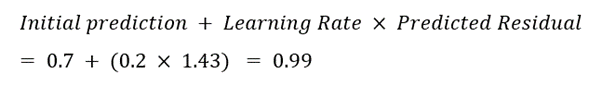
Let us consider the second observation in the dataset. Since, Good Blood Circulation = “Yes” followed by Blocked Arteries = “Yes” for the person, it ends up in the first leaf with a predicted residual of 1.43.
Assuming a learning rate of 0.2 , the new log(odds) prediction for this observation will be –
Next, we convert this new log(odds) into a probability value –
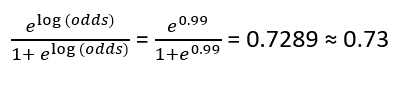
Similar computation is done for the rest of the observations.
V. Obtain new residuals — After obtaining the predicted probabilities for all the observations, we will calculate the new residuals by subtracting these new predicted values from the actual values.
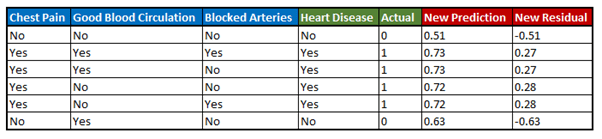
Fig 7. Sample dataset with residuals calculated using new predicted probabilities
Now that we have the residuals, we will use these leaves for building the next decision tree as described in step III.
VI. Repeat steps III to V until the residuals converge to a value close to 0 or the number of iterations matches the value given as hyperparameter while running the algorithm.
VII. Final Computation — After we have calculated the output values for all the trees, the final log(odds) prediction that a person has a heart disease will be the following –

where subscript of predicted residual denotes the i-th tree where i = 1,2,3,…
Next, we need to convert this log(odds) prediction into a probability by plugging it into the logistic function.
Using the common probability threshold of 0.5 for making classification decisions, if the final predicted probability that the person has a heart disease > 0.5, then the answer will be “Yes”, else “No”.
Hope these steps helped you understand the intuition behind working of GBT for classification !
Let us now keep a note of a few important parameters, pros, and cons of this method.
Important Parameters
While constructing any model using GBT, the values of the following can be tweaked for improvement in model performance –
- number of trees (n_estimators; def: 100)
- learning rate (learning_rate; def: 0.1) — Scales the contribution of each tree as discussed before. There is a trade-off between learning rate and number of trees. Commonly used values of learning rate lie between 0.1 to 0.3
- maximum depth (max_depth; def: 3) — Maximum depth of each estimator. It limits the number of nodes of the decision trees
Note — The names of these parameters in Python environment along with their default values are mentioned within brackets
Advantages
- It is a generalised algorithm which works for any differentiable loss function
- It often provides predictive scores that are far better than other algorithms
- ·It can handle missing data — imputation not required
Disadvantages
- This method is sensitive to outliers. Outliers will have much larger residuals than non-outliers, so gradient boosting will focus a disproportionate amount of its attention on those points. Using Mean Absolute Error (MAE) to calculate the error instead of Mean Square Error (MSE) can help reduce the effect of these outliers since the latter gives more weights to larger differences. The parameter ‘criterion’ helps you choose this function.
- It is prone to overfit if number of trees is too large. The parameter ‘n_estimators’ can help determining a good point to stop before our model starts overfitting
- Computation can take a long time. Hence, if you are working with a large dataset, always keep in mind to take a sample of the dataset (keeping odds ratio for target variable same) while training the model.
Conclusion
Although GBT is being widely used nowadays, many practitioners still use it as a complex black-box and just run the models using pre-built libraries. The purpose of this article was to break down the supposedly complex process into simpler steps and help you understand the intuition behind the working of GBT. Hope the post served its purpose !