Marketing Mix Modelling: What drives your ROI?

There was a time when we considered traditional marketing practices, and the successes or failures they yield, as an art form. With mysterious, untraceable results, marketing efforts lacked transparency and were widely regarded as being born out of the creative talents of star marketing professionals, but the dynamics switched, and regime of analytics came into power. It has evolved over the time and numerous methodologies have been discovered in this regard. Market mix model is one among those popular methods.
The key purpose of a Marketing Mix Model is to understand how various marketing activities are contributing together in driving the sales of any given product. Through MMM the effectiveness of each marketing input/channel can be assessed in terms of Return on Investment (ROI). In other words, a marketing input/channel with higher ROI is a more effective than others with a lower ROI. Such understanding facilitates effective marketing decisions with regards to spends allocation across channels.
Marketing Mix Modelling is a statistical technique of determining the effectiveness of marketing campaigns by breaking down aggregate data and differentiating between contributions from marketing tactics and promotional activities, and other uncontrollable drivers of success. It is used as a decision-making tool by brands to estimate the effectiveness of various marketing initiatives in increasing Return on Investment (ROI).
Whenever we change our methodologies, it is our human nature we would have various questions. Let’s deep dive into the MMM Modelling technique and address these questions in detail.
Question 1: How is the data collected? How much minimum data is required?
MMM Model requires a brand`s product data to collectively capture the impact of key drivers such as marketing spends, price factor, discounts, social media presence/sentiment of the product, event information etc. In any analytical method, more the data, better is the implementation of the modelling technique and more robust the results will be. Hence, these methods are highly driven by the quantum of data available to develop the model over.
Question 2: What level of data granularity is required/best for MMM?
A best practice for any analytical methodology and to generate valuable insights is to have as granular data as possible. For example, a Point-of-Sale data at Customer-Transaction-Item level will yield recommendations with highly focused marketing strategy at similar granularity. However, if needed, the data can always be rolled up at any aggregated level suitable for the business requirement.
Question 3: Which sales drivers are included in the marketing mix model?
In order to develop a robust and stable Market Mix Model, various sales drivers such as Price, Distribution, Seasonality, Macroeconomic variables, Brand Affinity etc. play a pivotal role in understanding the consumer behaviour towards product. Even more important are the features that capture the impact of marketing efforts for the product. Such features provide an insight into how consumers react to the respective marketing efforts or the impact of these efforts on the product.
Question 4: How do you ensure the accuracy of the data inputs?
Ensuring accuracy of data inputs is very subjective with respect to business. On many occasions direct imputation is not very helpful and would skew the results. Further sanity check and statistical testing like distribution of each feature set can be measured.
MMM Components –
In Market Mix Modelling sales are divided into 2 components:
Base Sales:
Base Sales is what marketers get if they do not do any advertisement. It is sales due to brand equity built over the years. Base Sales are usually fixed unless there is some change in economic or environmental factors.
Base Drivers:
- Price: The price of a product is a significant base driver of sales as price determines both the consumer segment that a product is targeted toward and the promotions which are implemented to market the product to the chosen audience.
- Distribution: The number of store locations, their respective inventories, and the shelf life of that stock are all considered as base drivers of the sales. Store locations and the inventory are static and can be unwittingly understood by customers without any marketing intervention.
- Seasonality: Seasonality refers to variations that occur in a periodic manner. Seasonal opportunities are enormous, and often they are the most commercially critical times of the year. For example, major share of electronics sales is around the holiday season.
- Macro-Economic Variables: Macro-economic factors greatly influence businesses and hence, their marketing strategies. Understanding of macro factors like GDP, unemployment rate, purchase power, growth rate, inflation and consumer sentiment is very critical as these factors are not under the control of businesses yet substantially impact them.
Incremental Sales:
This is sales generated by marketing activities like TV advertisement, print advertisement, and digital spends, promotions etc. Total incremental sales are split into sales from each input to calculate contribution to total sales.
Incremental Drivers:
- Media Ads: Promotional media ads form the core of MMM which penetrates the market and competitor deeply and create awareness about product key feature & other aspects. Numerous media channel available such as TV, print ads, digital ads, social media, direct mail marketing campaigns, in-store marketing etc.
- Product Launches: Marketers invest carefully to position the new product into the market and plan marketing strategies to support the new launch.
- Events & Conferences: Brands need to look for opportunities to build relationships with prospective customers and promote their product through periodic events and conferences.
- Behavioural Metrics: Variables like touch points, online behaviour metrics and repurchase rate provide deeper insights into customers for businesses.
- Social Metrics: Brand reach or recognition on social platforms like Twitter, Facebook, YouTube, blogs, and forums can be measured through indicative metrics like followers, page views, comments, views, subscriptions, and other social media data. Other social media data like the types of conversations and trends happening in your industry can be gathered through social listening.
Ad-stock Theory –
Ad-stock, or goodwill, is the cumulative value of a brand’s advertising at a given point in time. For example, if any company is advertising its product over 10 weeks, then for any given week t spending value would be X + Past Week Fractional Amount.
Ad-stock theory states that advertising is not immediate and has diminishing returns, meaning that its influential power decreases over time, even if more money is allocated to it. Therefore, time regression analysis will help marketers to understand the potential timeline for advertising effectiveness and how to optimize the marketing mix to compensate for these factors

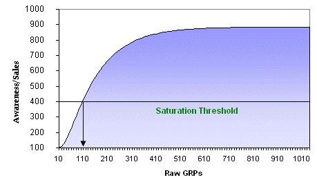
- Diminishing Returns: The underlying principle for TV advertisement is that the exposure to TV ads create awareness to a certain extent in the customers’ minds. Beyond that, the impact of exposure to ads starts diminishing over time. Each incremental amount of GRP (stand for “Gross Rating Point” which measures impact of Advertisement) would have a lower effect on Sales or awareness. So, the incremental sales generated from incremental GRP start to diminish and saturate eventually. This effect can be seen in the above graph, where the relationship between TV GRP and sales in non-linear. This type of relationship is captured by taking exponential or log of GRP.
- Carry over effect or Decay Effect: The impact of past advertisement on present sales is known as Carry over effect. A small component termed as lambda is multiplied with the past month GRP value. This component is also known as Decay effect as the impact of previous months’ advertisement decays over time.

Implementation details:
The most common marketing mix modelling regression techniques used are:
- Linear regression
- Multiplicative regression
1. Linear Regression Model:
Linear regression can be applied when the DV is continuous and the relationship between the DV and IDVs is assumed to be linear. The relationship can be defined using the equation:

Here ‘Sales’ is the dependent variable to be estimated, X are the independent variables and ε is the error term. βi’s are the regression coefficients. The difference between the observed outcome Sales and the predicted outcome sales is known as a prediction error. Regression analysis is mainly used for Causal analysis, Forecasting the impact of a change, Forecasting trends etc. However, this method does not perform well on large amounts of data as it is sensitive to outliers, multicollinearity, and cross-correlation.
2. Multiplicative Regression Models-
Additive models imply a constant absolute effect of each additional unit of explanatory variables. They are suitable only if businesses occur in more stable environments and are not affected by interaction among explanatory variables. But in scenarios such as when pricing is zero, the sales (DV) will become infinite.
To overcome the limitations inherent in linear models, multiplicative models are often preferred. These models offer a more realistic representation of reality than additive linear models do. In these models, IDVs are multiplied together instead of added.
There are two kinds of multiplicative models:
Semi-Logarithmic Models-
In Log-Linear models, the exponents of independent variables are multiplied.

Logarithmic transformation of the target variable linearizes the model form, which in turn can be estimated as an additive model. The dependent variable is logarithmic transformed, the only difference between additive model and semi-logarithmic model

Some of the benefits of Log-Linear models are:
- The coefficients β can be interpreted as % change in business outcome (sales) to unit change in the independent variables.
- Each independent variable in the model works on top of what has been already achieved by other drivers.
Logarithmic Models-
In Log-Log models, independent variables are also subjected to logarithmic transformation in addition to the target variable.

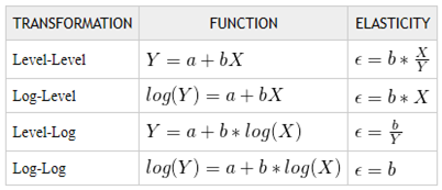
In the case of non-linear regression models, the above defined elasticity formula needs to be tweaked according to the equation. Refer the table below.

Statistical significance –
Once the model has been generated, it should be checked for validity and prediction quality. Based on the nature of the problem, various model stats are used for evaluation purposes. The following are the most common statistical measures in marketing mix modelling
- R-squared – R-squared is a statistical measure of how close the data are to the fitted regression line. It is also known as the coefficient of determination. R-squared is always between 0 and 100%; 0% indicates that the model explains none of the variability of the response data around its mean.100% indicates that the model explains all the variability of the response data around its mean. General formula for R-squared is: R2 = 1 – Where SSE = Sum of squared errors and SST = Total sum of square
- Adjusted R Squared: The adjusted R-squared is a refined version of R-squared that has been penalized for the number of predictors in the model. It increases only if the new predictor improves the model. The adjusted R-squared can be used to compare the explanatory power of regression models that contain different numbers of predictors.
- Coefficient: Regression coefficients are estimates of the unknown population parameters and describe the relationship between a predictor variable and the response. In linear regression, coefficients are the values that multiply the predictor values. The sign of each coefficient indicates the direction of the relationship between a predictor variable and the response variable. A positive sign indicates that as the predictor variable increases, the response variable also increases. A negative sign indicates that as the predictor variable increases, the response variable decreases
- Variable Inflation Factor: A variance inflation factor (VIF) detects multicollinearity in regression analysis. Multicollinearity is when there is a correlation between predictors (i.e. independent variables) in a model. The VIF estimates how much the variance of a regression coefficient is inflated due to multicollinearity in the model. Every variable in the model would be regressed against all the other available variables to calculate the VIF. VIF is usually calculated as Where Ri2 is R-squared value obtained by regressing “i”, the predictor variable against all other variables.
- Mean Absolute Error (MAE): MAE measures the average magnitude of the errors in a set of predictions. It is the average over the absolute differences between prediction and actual observation where all individual differences have equal weight Where Yt is the actual value at time ‘t’ and ŷt is the predicted value at time ‘t’
- Mean Absolute Percentage Error (MAPE): MAPE is the average absolute percent error for each observation or predicted values minus actuals divided by actuals Where yt is the actual value at time ‘t’ and ŷt is the predicted value at time ‘t’
MMM Output –

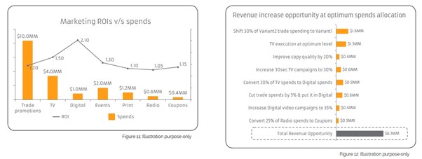
Marketing Mix Model outputs provide contribution of each marketing vehicle/channel, which along with marketing spends, provide marketing ROIs. It also captures time decay and diminishing returns on different media vehicles, as well as the effects of other non-marketing factors discussed above and other interactions like the halo effect and cannibalization. The model output provides all the necessary components and parameters required to arrive at the best media mix under any condition
Expected Benefit & Limitation –
Benefits of Marketing Mix Modelling –
- Enables marketers to prove the ROI of their efforts across marketing channels
- Returns insights that allow for effective budget allocation
- Facilitates superior sales trend forecasting
Limitations of Marketing Mix Modelling –
- Lacks the convenience of real-time modern data analytics
- Critics argue that modern attribution methods are more effective as they consider 1 to 1, individual data
- Marketing Mix Modelling does not analyze customer experience (CX)
Application/Scope for Optimization, Extension of MMM Model
1. Scope for Optimization
Marketing optimization is the process of improving marketing efforts to maximize desired business outcomes. Since the nature of MMM are mostly non-linear, non-linear constrained algorithms are used for optimization. Some of the use cases for marketing mix optimization are:
To improve current sales level by x%, what is the level of spends required in different marketing channels? E.g., To increase sales by 10%, how much to invest in TV ads or discounts or sales promotions?
What happens to the outcome metric (sales, revenue, etc.), if the current level of spends is increased by x%? E.g., On spending additional $20M on TV, how much more sales can be obtained? Where are these additional spends to be distributed?
2. Halo and Cannibalization Impact
Halo effect is a term for a consumer’s favouritism towards a product from a brand because of positive experiences they have had with other products from the same brand. Halo effect can be the measure of a brand’s strength and brand loyalty. For example, consumers favour Apple iPad tablets based on the positive experience they had with Apple iPhones.
Cannibalization effect refers to the negative impact on a product from a brand because of the performance of other products from the same brand. This mostly occurs in cases when brands have multiple products in similar categories. For example, a consumer’s favouritism towards iPads can cannibalize MacBook sales.
In Marketing Mix Models, base variables, or incremental variables of other products of the same brand are tested to understand the halo or cannibalizing impact on the business outcome of the product under consideration.
Conclusion
Marketing mix modelling techniques can minimize much of the risk associated with new product launches or expansions. Developing a comprehensive marketing mix model can be the key to sustainable long-term growth for a company. It will become a key driver for business strategy and can improve the profitability of a
company’s marketing initiatives. While some companies develop models through their in-house marketing and analytics departments, many choose to collaborate with an external company to develop the most efficient model for their business.
Developers of marketing mix models need to have a complete understanding of the marketing environment they operate within and of the latest advanced market research techniques. Only through this will they be able to fully comprehend the complexities of the numerous marketing variables that need to be accounted for and calculated in a marketing mix model. While numerical and statistical expertise is undoubtedly crucial, an insightful understanding of market research and market environments is just as important to develop a holistic and accurate marketing mix model. With these techniques, you can get started on developing a watertight marketing mix model that can maximise performance and sales of a new product.
References:
- https://towardsdatascience.com/market-mix-modeling-mmm-101-3d094df976f9
- https://www.listendata.com/2019/09/marketing-mix-modeling.html
- https://cartesianconsulting.com/wp-content/uploads/2017/06/Cartesian-MMM-Playbook-Mar-2017-LR.pdf
- https://www.nielsen.com/eu/en/solutions/capabilities/marketing-mix-modeling/
- https://www.exlservice.com/market-mix-modeling-for-retail