Month: October 2021 - Page 2

The Evolution of Movies : How has it changed with time?

Posted on October 29, 2021June 23, 2023 by affine

“Cinema is a mirror by which we often see ourselves.” – Alejandro Gonzalez Inarritu

If 500 people saw a movie, there exist 500 different versions of the same idea conveyed by the movie. Often movies reflect culture, either what the society is or what it aspires to be.

From “Gone with the Wind” to “Titanic” to “Avengers: Endgame,” Movies have come a long way. The Technology, Scale, and Medium might have changed, but the essence has remained invariable to storytelling. Any idea or story that the mind can conceive can be given life in the form of Movies.

The next few minutes would be a humble attempt to share the What, Why, and How of the Movie Industry.

Sections:

The process behind movies
How did the movie industry operate?
How is it functioning now?
What will be the future for movies?

1. The process behind movies

We see the end output in theatres or in the comfort of our homes (on Over-The-Top (OTT) platforms like Netflix, Amazon Prime, HBO Max, etc.). But in reality, there is a long and ardent process behind movie-making.

As with all things, it starts with an idea, an idea that transcribes into a story, which then takes the form of a script detailing the filmmaker’s vision scene by scene.

They then pitch this script to multiple studios (Disney, Universal, Warner Bros., etc.). When a studio likes this script, they decide to make the film using its muscle for pre-production, production, and post-production.

The filmmaker and studio start with the pre-production activities such as hiring cast and crew, choosing filming locations to set constructions. Post which the movie goes into the production phase, where it gets filmed. In post-production, the movie gets sculpted with music, visual effects, video & sound editing, etc.

And while moviemakers often understand the art of movie-making, it becomes a product to be sold on completing production. Now they have to sell this story to the audience.

Marketing & distribution step in to ensure that this product is now available to its worldwide audience by promoting it in all possible mediums like billboards and social media. After this, it’s all about delivering an immersive, entertaining experience where your surroundings go dark and the mind lights up.

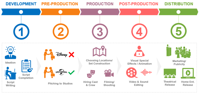
An Overview Of The Movie-Making Process

In recent times some creative flexibility has been observed in the above process. For example, studios who own certain characters or intellectual property like Marvel & DC characters hire the right talent to get their movies made. In such cases, big studios control significant aspects of the film, from content creation to distribution.

2. How did the movie industry operate?

For a considerable period, movies used to stay in theatres for a long time post their initial release before reaching other available forms of Home Entertainment (based on the technological choices/era). For example, Let’s take a movie that acted as the bridge between two distinct generations. Titanic transformed the industry from the old school blockbusters to the new school global hits (with technology, CGI, worldwide markets, etc.) And before the 2010s, blockbuster movies like Titanic used to run in theatres for several months. Titanic was the undisputed leader of Box Office for nearly four months, both in terms of the number of tickets sold and worldwide revenue generated.

Post its theatrical run of approximately four months, blockbuster titles used to be available in-Home Entertainment (HE) formats (such as DVD, VCD, etc.) These formats were available in various options based on the decade or era. Options such as rental or purchasable DVDs ruled the HE domain for a considerable amount of time. Until the emergence of the internet.

The Dawn of the internet brought in other sources of entertainment in competition to the traditional Movies, Sports, etc. These options gave the consumer alternate forms of entertainment (which resulted in shortened theatrical runs, approximately three months or less). They gave the studios also another platform to sell their content. Hence the Home Entertainment release windows were fast-tracked as a natural consequence to capitalize the most from the movie’s potential.

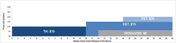
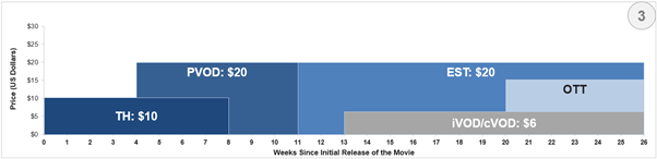
The following is an example of the pre-2020/pandemic norms in Hollywood.

December 25: Movie releases in Theatres (TH). Ex: Fast and Furious March 10 19: EST (Electronic Sell Through) release of the movie (Ex: Amazon, iTunes)
April 2: iVOD/cVOD (Internet/Cable Video on Demand) release of the movie (Ex: YouTube, Comcast, Amazon)
April 30: PST (Physical Sell Through) release of the movie (Ex: DVDs, Blu-ray discs)
After this, the movie becomes available on Linear TV networks (Ex: HBO)

An Overview Of Movie Releases Before And After Pandemic

3. How is it functioning now?

Amid all the uncertainty surrounding the COVID pandemic, the movie industry did come to a halt, as did many other integral aspects of people’s lives. Around March 2020, most theatres worldwide shut down to prevent the widespread pandemic. The forceful shutting of the movie industry immobilized crucial aspects of the filmmaking process, such as the filming & theatrical release of movies. Since it was not safe for people to gather in numbers, theatres closed, as did other forms of entertainment such as Concerts, Live Sports, etc. This change of unprecedented magnitude was the first since world wars, where major entertainment activities worldwide were shut down.

With every problem, there lies an opportunity, as with this change, innovation was the name of the game. Those businesses that innovated survived, and the rest were likely to perish. The founding stone for this innovation was laid a long time back. With the influx of the internet, OTT (Over-The-Top) & VOD (Video on Demand) platforms were rapidly growing. OTT Platforms like Netflix & Amazon Prime were significant players in the US and worldwide before the beginning of the pandemic itself.

Shutting down of theatres meant some movies slated for 2020 waited for release dates. In the movie industry, movies are often planned well in advance. Major studios are likely to have tentative release dates for the upcoming 2 to 3 years. Delaying movies of the current year not only does it cumulatively delay the subsequent year’s release dates, but it also decays the potential of the film (due to factors like heavy competition later, loss of audience interest, etc.)

Major studios & industry leaders lead the way with innovation. A new format (Premium Video on Demand) and a new release strategy were the most viable options to ensure the movie’s release, guaranteeing both financial and viewership success.

The New Format – PVOD (Premium Video on Demand) was essentially releasing the iVOD/cVOD rental formats at an earlier period by shortening the pre-pandemic normal of 12 weeks post-theatrical release window to an earlier release window.

There were two ways of doing this; the first one is a Day and Date release in PVOD, which meant the audience can watch a new movie (Ex: Trolls World Tour, Scoob!) on its first release date at the comfort of their homes via the PVOD/rental channels (Ex: Amazon/iTunes)

The second way for the PVOD format is by releasing the movie in PVOD 2 to 8 weeks post its release in theatres. This happened once people got used to the new normal during the pandemic. Theatres across the world opened partially with limited seating capacity (50%). This meant that a movie would release in theatres exclusively first (as it was previously). However, the traditional Home Entertainment window of 12 weeks bypassed to release PVOD at an early window of 2 to 8 weeks post Theatrical release. This was the key in catering to a cautious audience during the pandemic between 2020 to 2021. This enabled them to watch a newly released movie at the comfort of their homes within a couple of weeks of its initial release itself.

A similar strategy was also tried with EST, where an early EST release (Premium EST or PEST) is offered to people at an early release window. The key difference is that PEST and PVOD were sold at higher price points (25% higher than EST/iVOD/cVOD) due to their exclusivity and early access.

The other strategy was a path-breaking option that opened the movie industry to numerous viable release possibilities – a direct OTT release. A movie waiting for its release & does not want to use the PVOD route due to profitability issues, or other reasons can now release the film directly on OTT platforms like Netflix & Amazon Prime. These platforms, which were previously producing small to medium-scale series & movies, now have the chance to release potential blockbuster movies on their platform. Studios also get to reach Millions of customers across the globe at the same time by jumping certain cumbersome aspects posed by the conventional theatrical distribution networks (which includes profit-sharing mechanisms). In this route of OTT platform release, there are many advantages to all parties involved (Studios, OTT Platforms & Audiences) and the number of potential customers.

The studios either get a total remuneration paid for the movie upfront (e.g., Netflix made a $200 Million offer for Godzilla vs. Kong to its producers, Legendary Entertainment & Warner Bros.). Or get paid later based on the number of views gathered in a given period or a combination of both (depending upon the scale & genre of the movie). The OTT platforms will now have a wide array of the latest movies across all genres to attract & retain customers. The people will now get to watch new movies on their preferred OTT platforms at their convenience and get a great value for money spent (OTT 1-month subscription ~$10 for new movie + existing array of movies & series vs. ~ $10 Theatre Ticket Price for one movie)

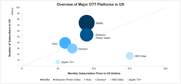
Overview of Major OTT Platform in US

Given there are two new gateways (OTT & PVOD) to release films in addition to the existing conventional mediums such as Theatres, EST, iVOD, cVOD, PST. There are numerous beneficial ways a movie can be released to reach the maximum people & make the most profit for the filmmakers & studios.

Release Strategy Examples

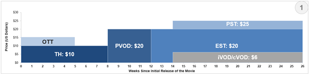
In the above example, releasing a movie directly in OTT in parallel to theatrical release attracts more subscribers to the OTT platform and covers the traditional theatrical audiences.

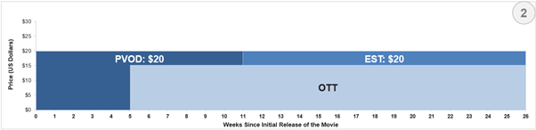
In the second example, let’s take a direct to Home Entertainment approach, targeting audiences directly in PVOD & early OTT releases. Similar to the movies that were released during the pandemic, like Trolls World Tour & Scoob!

The third example shows a possibility where a movie can leverage all existing major platforms for a timely release.

Since there are hundreds of possibilities for any studio or filmmaker to release their movies, how would one know the best release strategy for a movie? Does one size fit all methods work? Or do we scale and change release strategies according to the Budget/Content of the movie? Are certain genre films more suited for large-scale theater experience than being better suited for Home Entertainment? Who decides this? That should be a straightforward answer. In most cases, the one who finances the film decides the release strategy. But how would they know what combination ensures the maximum success to recoup the amount invested and guarantee a profit for all involved?

In such an uncertain industry, where more movies fail than succeed (considering the bare minimum of breaking even), the pandemic-induced multiple release strategies compound the existing layers of complexity.

In an ocean of uncertainties, the ship with a compass is likely to reach the shore safely. The compass, in this case, is Analytics. Analytics, Insights & Strategy provide the direction to take the movie across to the shores safely and profitably.

Analytics, Insights & Strategy (AIS) helps deal with the complex nature of movies and provides a headstrong direction for decision making, be it from optimal marketing spend recommendations to profitable release strategies. There are thousands of films with numerous data points. When complex machine learning models leverage all this data, it yields eye-opening insights for the industry leaders to make smart decisions. Capitalizing on such forces eases the difficulties in creating an enjoyable & profitable movie.

4. What will be the future for movies?

The Entertainment industry evolves as society progresses forward. Movies & theatres have stood the test of time for decades. There will always be a need for a convincing story, and there will always be people to appreciate good stories. Although with what seems to be a pandemic-induced shift into the world of online entertainment & OTT’s. This change was inevitable and fast-tracked due to unexpected external factors.

What the future holds for this industry is exciting for both the filmmakers and the audiences. The audiences have the liberty to watch movies across their preferred mediums early on, rather than the conventional long drawn theatrical only way. The studios now have more ways to engage audiences with their content. In addition to the theatrical experience, they can reach more people faster while ensuring they run a profitable business.

We will soon start seeing more movies & studios using the OTT platforms for early releases and the conventional theatre first releases with downstream combinations of other Home Entertainment forms to bring the movie early to the audience on various platforms.

On an alternate note, in the future, we might be in a stage where Artificial Intelligence (AI) could be generating scripts or stories based on user inputs for specific genres. An AI tool could produce numerous scripts for filmmakers to choose from. It is exciting to think of its potential, for example, say in the hands of an ace director like Christopher Nolan with inputs given to the AI tool based on movies like Tenet or Inception.

Post-Pandemic, when life returns to normal, we are likely to see star-studded, big-budget movies directly being released on Netflix or HBO Max, skipping the conventional theatrical release. Many filmmakers have expressed concerns that the rise of OTT may even lead to the death of theatres.

That said, I do not think that the theatres would perish. Theatres were and will always be a social experience to celebrate larger-than-life movies. The number of instances where people go to theatres might reduce since new movies will be offered in the comfort of their homes.

With all this discussion surrounding making profitable movies, with the help of Analytics, Insights & Strategy, why don’t filmmakers and studios stop after making a couple of profitable movies?

The answer is clear, as stated by Walt Disney, one of the brightest minds of the 20th century, “We don’t make movies to make money, we make money to make more movies.”

References:

Hotel Recommendation Systems: What is it and how to effectively build one?

Posted on October 29, 2021March 9, 2023 by affine

What is a Hotel Recommendation System?

A hotel recommendation system aims at suggesting properties/hotels to a user such that they would prefer the recommended property over others.

Why is a Hotel Recommendation System required?

In today’s data-driven world, it would be nearly impossible to follow the traditional heuristic approach to recommend millions of users an item that they would actually like and prefer.

Hence, a Recommendation System solves our problem where it incorporates user’s input, historical interaction, and sometimes even user’s demographics to build an intelligent model to provide recommendations.

Objective:

In this blog, we will cover all the steps that are required to build a Hotel Recommendation System for the problem statement mentioned below. We will do an end-to-end implementation from data understanding, data pre-processing, and the algorithms used along with their PySpark codes.

Problem Statement: Build a recommendation system providing hotel recommendations to users for a particular location they have searched for on xyz.com

What type of data are we looking for?

Building a recommendation system requires two sources of data, explicit and implicit signals.

Explicit data is the user’s direct input, like filters (4 star rated hotel or preference of pool in a hotel) that a user applies while searching for a hotel. Information such as age, gender, and demographics also comes under explicit signals.

Implicit data can be obtained by users’ past interactions, for example, the average star rating preferred by the user, the number of times a particular hotel type (romantic property) is booked by the user, etc.

What data are we going to work with?

We are going to work with the following:

Explicit signals where a user provides preferences for what type of amenities they are looking for in a property
Historical property bookings of the user
Users’ current search results from where we may or may not get information regarding the hotel that a user is presently interested in

Additionally, we have the property information table (hotel_info table), which looks like the following:

hotel_info table

Note: We can create multiple property types (other than the above 4, Wi-Fi, couple, etc.) ingeniously covering the maximum number of properties in at least one of the property types. However, for simplicity, we will continue with these 4 property types.

Data Understanding and Preparation:

Consider that the searches data is in the following format:

user_search table

Understanding user_search table:

Information about a user (user ID), the location they are searching in (Location ID), their check-in and check-out dates, the preferences applied while making the search (Amenity Filters), the property specifically looked into while searching (Property ID), and whether they are about to book that property (Abandoned cart = ‘yes’ means that they are yet to make the booking and only the payment is left) can be extracted from the table

Clearly, we do not have all the information for the searches made by the user hence, we are going to split the users into 3 categories; namely, explicit users (users whose amenity filter column is not null), abandoned users (users whose abandoned cart column is ‘yes’), and finally, historical users (users for whom we have historical booking information)

Preparing the data:

For splitting the users into the 3 categories (explicit, abandoned, historical), we give preference in the following order, Abandoned users>Explicit users>historical users. This preferential order is because of the following reasons:

The abandoned cart gives us information regarding the product the user was just about to purchase. We can exploit this information to give recommendations similar to the product in the cart; since the abandoned product represents what a user prefers. Hence, giving abandoned users the highest priority.

An explicit signal is an input directly given by the user. The user directly tells his preference through the Amenities column. Hence, explicit users come next in the order.

Splitting the users can be done following the steps below:

Firstly, create a new column as user_type, under which each user will be designated with one of the types, namely, abandoned, explicit, or historical

Creating a user_type column can be done using the following logic:

df_user_searches = spark.read.parquet(‘xyz…….’)

df_abandon = df_user_searches.withColumn(‘abandon_flag’,F.when(col(‘Abandon_cart’).like(‘yes’) & ‘Property_ID is not Null’,lit(1)).otherwise(lit(None))).filter(‘abandon_flag = 1’).withColumn(‘user_type’,lit(‘abandoned_users’)).drop(‘abandon_flag’)

df_explicit = df_user_searches.join(df_abandon.select(‘user_ID’),’user_ID’,’left_anti’).withColumn(‘expli_flag’,F.when(col(‘Amenity_Filters’).like(‘%Wifi Availibility%’)|col(‘Amenity_Filters’).like(‘%Nature Friendly%’)|col(‘Amenity_Filters’).like(‘%Budget Friendly%’)|col(‘Amenity_Filters’).like(‘%Couple Friendly%’),lit(1)).otherwise(lit(None))).filter(‘expli_flag = 1’).withColumn(‘user_type’,lit(‘explicit_users’)).drop(‘expli_flag’)

df_historical = df_user_searches.join(df_abandon.unionAll(df_explicit).select(‘user_ID’).distinct(),’user_ID’,’left_anti’).withColumn(‘user_type’,lit(‘historical_user’))

df_final = df_explicit.unionAll(df_abandon).unionAll(df_historical)

Now, the user_search table has the user_type as well. Additionally,

For explicit users, user_feature columns will look like this:

explicit_users_info table

For abandoned users, after joining the property id provided by the user with that in the hotel_info table, the output will resemble as follows:

abandoned_users_info table

For historical users, sum over the user and calculate the total number of times the user has booked a particular property type; the data will look like the following:

historical_users_info table

For U4 in the historical_users_info table, we have information that tells us that the user prefers an average star rating of 4, has booked WiFi property 5 times, and so on. Eventually, telling us the attribute preferences of the user….

Building the Recommendation System:

Data at hand:

We have users split and user’s preferences as user_features

We have the hotel attributes from the hotel_type table, assume that it contains the following values:

hotel_type table

We will use content-based-filtering in building our recommendation model. For each of the splits, we will use an algorithm that will give us the best result. To gain a better understanding of recommendation systems and content-based filtering, one can refer here.

Note: We have to give recommendations based on the location searched by the user. Hence, we will perform a left join on the key Location ID to get all the properties that are there in the location.

Building the system:

For Explicit users, we will proceed in the following way:

We have user attributes like wifi_flag, budget_flag, etc. Join this with the hotel_type table on the location ID key to get all the properties and their attributes

Performing Pearson correlation will give us a score([-1,1]) between the user and hotel features, eventually helping us to provide recommendation in that location

Code for explicit users:

explicit_users_info = explicit_users_info.drop(‘Property_ID’)

expli_dataset = explicit_users_info.join(hotel_type,[‘location_ID’],’left’).drop(‘star_rating’)

header_user_expli = [‘wifi_flag’,’couple_flag’,’budget_flag’,’nature_flag’]

header_hotel_features = [‘Wifi_Availibility’,’Couple_Friendly’,’Budget_Friendly’,’Nature_Friendly’]

assembler_features = VectorAssembler(inputCols= header_user_expli, outputCol=”user_features”)

assembler_features_2 = VectorAssembler(inputCols= header_hotel_features, outputCol=”hotel_features”)

tmp = [ assembler_features,assembler_features_2]

pipeline = Pipeline(stages=tmp)

baseData = pipeline.fit(expli_dataset).transform(expli_dataset)

df_final = baseData

def pearson(a,b):

if (np.linalg.norm(a) * np.linalg.norm(b)) !=0:

a_avg, b_avg = np.average(a), np.average(b)

a_stdev, b_stdev = np.std(a), np.std(b)

n = len(a)

denominator = a_stdev * b_stdev * n

numerator = np.sum(np.multiply(a-a_avg, b-b_avg))

p_coef = numerator/denominator

return p_coef.tolist()

pearson_sim_udf = udf(pearson, FloatType())

pearson_final = df_final.withColumn(‘pear_correlation_res’, pearson_sim_udf(‘user_features’,’hotel_features’))

pearson_final.withColumn(‘recommendation_rank’,F.row_number().over(Window.partitionBy(‘User_ID’).orderBy(desc(‘pear_correlation_res’)))).show()

Our output will look like the following:

explicit users

For abandoned and historical users, we will proceed as follows:

Using the data created above, i.e., abandoned_users_info and historical_users_info tables, we obtain user preferences in the form of WiFi_Availibility or wifi_flag, star_rating or avg_star_rating, and so on

Join it with the hotel_type table on the location ID key to get all the hotels and their attributes

Perform Cosine Similarity to find the best hotel to recommend to the user in that particular location

Code for abandoned users:

abandoned_users_info = abandoned_users_info.drop(‘Property_ID’)\

.withColumnRenamed(‘Wifi_Availibility’,’a_Wifi_Availibility’)\

.withColumnRenamed(‘Nature_Friendly’,’a_Nature_Friendly’)\

.withColumnRenamed(‘Budget_Friendly’,’a_Budget_Friendly’)\

.withColumnRenamed(‘Couple_Friendly’,’a_Couple_Friendly’)\

.withColumnRenamed(‘Star_Rating’,’a_Star_Rating’)

abandoned_dataset = abandoned_users_info.join(hotel_type,[‘location_ID’],’left’)

header_user_aban = [‘a_Wifi_Availibility’,’a_Couple_Friendly’,’a_Budget_Friendly’,’a_Nature_Friendly’,’a_Star_Rating’]

header_hotel_features = [‘Wifi_Availibility’,’Couple_Friendly’,’Budget_Friendly’,’Nature_Friendly’,’Star_Rating’]

assembler_features = VectorAssembler(inputCols= header_user_aban, outputCol=”user_features”)

assembler_features_2 = VectorAssembler(inputCols= header_hotel_features, outputCol=”hotel_features”)

tmp = [ assembler_features,assembler_features_2]

pipeline = Pipeline(stages=tmp)

baseData = pipeline.fit(abandoned_dataset).transform(abandoned_dataset)

df_final = baseData

def cos_sim(value,vec):

if (np.linalg.norm(value) * np.linalg.norm(vec)) !=0:

dot_value = np.dot(value, vec) / (np.linalg.norm(value)*np.linalg.norm(vec))

return dot_value.tolist()

cos_sim_udf = udf(cos_sim, FloatType())

abandon_final = df_final.withColumn(‘cosine_dis’, cos_sim_udf(‘user_features’,’hotel_features’))

abandon_final.withColumn(‘recommendation_rank’,F.row_number().over(Window.partitionBy(‘User_ID’).orderBy(desc(‘cosine_dis’)))).show()

Code for historical users:

historical_dataset = historical_users_info.join(hotel_type,[‘location_ID’],’left’)

header_user_hist = [‘wifi_flag’,’couple_flag’,’budget_flag’,’nature_flag’,’avg_star_rating’]

header_hotel_features = [‘Wifi_Availibility’,’Couple_Friendly’,’Budget_Friendly’,’Nature_Friendly’,’Star_Rating’]

assembler_features = VectorAssembler(inputCols= header_user_hist, outputCol=”user_features”)

assembler_features_2 = VectorAssembler(inputCols= header_hotel_features, outputCol=”hotel_features”)

tmp = [ assembler_features,assembler_features_2]

pipeline = Pipeline(stages=tmp)

baseData = pipeline.fit(historical_dataset).transform(historical_dataset)

df_final = baseData

def cos_sim(value,vec):

if (np.linalg.norm(value) * np.linalg.norm(vec)) !=0:

dot_value = np.dot(value, vec) / (np.linalg.norm(value)*np.linalg.norm(vec))

return dot_value.tolist()

cos_sim_udf = udf(cos_sim, FloatType())

historical_final = df_final.withColumn(‘cosine_dis’, cos_sim_udf(‘user_features’,’hotel_features’))

historical_final.withColumn(‘recommendation_rank’,F.row_number().over(Window.partitionBy(‘User_ID’).orderBy(desc(‘cosine_dis’)))).show()

Our output will look like the following:

historical users

abandoned users

Giving Recommendations:

Giving 3 recommendations per user, our final output will look like the following:

Note:

One can notice that we are not using hotel recommendation X for the abandoned user U1 as a first recommendation we are avoiding so as hotel features were created from the same property ID, hence, it will always be at rank 1

Unlike cosine similarity where 0’s are considered a negative preference, Pearson correlation does not penalize the user if no input is given; hence we use the latter for explicit users

Conclusion:

In the end, the objective is to fully understand the problem statement, work around the data available, and provide recommendations with a nascent system.

Marketing Mix Modelling: What drives your ROI?

Posted on October 29, 2021March 9, 2023 by affine

There was a time when we considered traditional marketing practices, and the successes or failures they yield, as an art form. With mysterious, untraceable results, marketing efforts lacked transparency and were widely regarded as being born out of the creative talents of star marketing professionals, but the dynamics switched, and regime of analytics came into power. It has evolved over the time and numerous methodologies have been discovered in this regard. Market mix model is one among those popular methods.

The key purpose of a Marketing Mix Model is to understand how various marketing activities are contributing together in driving the sales of any given product. Through MMM the effectiveness of each marketing input/channel can be assessed in terms of Return on Investment (ROI). In other words, a marketing input/channel with higher ROI is a more effective than others with a lower ROI. Such understanding facilitates effective marketing decisions with regards to spends allocation across channels.

Marketing Mix Modelling is a statistical technique of determining the effectiveness of marketing campaigns by breaking down aggregate data and differentiating between contributions from marketing tactics and promotional activities, and other uncontrollable drivers of success. It is used as a decision-making tool by brands to estimate the effectiveness of various marketing initiatives in increasing Return on Investment (ROI).

Whenever we change our methodologies, it is our human nature we would have various questions. Let’s deep dive into the MMM Modelling technique and address these questions in detail.

Question 1: How is the data collected? How much minimum data is required?

MMM Model requires a brand`s product data to collectively capture the impact of key drivers such as marketing spends, price factor, discounts, social media presence/sentiment of the product, event information etc. In any analytical method, more the data, better is the implementation of the modelling technique and more robust the results will be. Hence, these methods are highly driven by the quantum of data available to develop the model over.

Question 2: What level of data granularity is required/best for MMM?

A best practice for any analytical methodology and to generate valuable insights is to have as granular data as possible. For example, a Point-of-Sale data at Customer-Transaction-Item level will yield recommendations with highly focused marketing strategy at similar granularity. However, if needed, the data can always be rolled up at any aggregated level suitable for the business requirement.

Question 3: Which sales drivers are included in the marketing mix model?

In order to develop a robust and stable Market Mix Model, various sales drivers such as Price, Distribution, Seasonality, Macroeconomic variables, Brand Affinity etc. play a pivotal role in understanding the consumer behaviour towards product. Even more important are the features that capture the impact of marketing efforts for the product. Such features provide an insight into how consumers react to the respective marketing efforts or the impact of these efforts on the product.

Question 4: How do you ensure the accuracy of the data inputs?

Ensuring accuracy of data inputs is very subjective with respect to business. On many occasions direct imputation is not very helpful and would skew the results. Further sanity check and statistical testing like distribution of each feature set can be measured.

MMM Components –

In Market Mix Modelling sales are divided into 2 components:

Base Sales:

Base Sales is what marketers get if they do not do any advertisement. It is sales due to brand equity built over the years. Base Sales are usually fixed unless there is some change in economic or environmental factors.

Base Drivers:

Price: The price of a product is a significant base driver of sales as price determines both the consumer segment that a product is targeted toward and the promotions which are implemented to market the product to the chosen audience.
Distribution: The number of store locations, their respective inventories, and the shelf life of that stock are all considered as base drivers of the sales. Store locations and the inventory are static and can be unwittingly understood by customers without any marketing intervention.
Seasonality: Seasonality refers to variations that occur in a periodic manner. Seasonal opportunities are enormous, and often they are the most commercially critical times of the year. For example, major share of electronics sales is around the holiday season.
Macro-Economic Variables: Macro-economic factors greatly influence businesses and hence, their marketing strategies. Understanding of macro factors like GDP, unemployment rate, purchase power, growth rate, inflation and consumer sentiment is very critical as these factors are not under the control of businesses yet substantially impact them.

Incremental Sales:

This is sales generated by marketing activities like TV advertisement, print advertisement, and digital spends, promotions etc. Total incremental sales are split into sales from each input to calculate contribution to total sales.

Incremental Drivers:

Media Ads: Promotional media ads form the core of MMM which penetrates the market and competitor deeply and create awareness about product key feature & other aspects. Numerous media channel available such as TV, print ads, digital ads, social media, direct mail marketing campaigns, in-store marketing etc.
Product Launches: Marketers invest carefully to position the new product into the market and plan marketing strategies to support the new launch.
Events & Conferences: Brands need to look for opportunities to build relationships with prospective customers and promote their product through periodic events and conferences.
Behavioural Metrics: Variables like touch points, online behaviour metrics and repurchase rate provide deeper insights into customers for businesses.
Social Metrics: Brand reach or recognition on social platforms like Twitter, Facebook, YouTube, blogs, and forums can be measured through indicative metrics like followers, page views, comments, views, subscriptions, and other social media data. Other social media data like the types of conversations and trends happening in your industry can be gathered through social listening.

Ad-stock Theory –

Ad-stock, or goodwill, is the cumulative value of a brand’s advertising at a given point in time. For example, if any company is advertising its product over 10 weeks, then for any given week t spending value would be X + Past Week Fractional Amount.

Ad-stock theory states that advertising is not immediate and has diminishing returns, meaning that its influential power decreases over time, even if more money is allocated to it. Therefore, time regression analysis will help marketers to understand the potential timeline for advertising effectiveness and how to optimize the marketing mix to compensate for these factors

Diminishing Returns: The underlying principle for TV advertisement is that the exposure to TV ads create awareness to a certain extent in the customers’ minds. Beyond that, the impact of exposure to ads starts diminishing over time. Each incremental amount of GRP (stand for “Gross Rating Point” which measures impact of Advertisement) would have a lower effect on Sales or awareness. So, the incremental sales generated from incremental GRP start to diminish and saturate eventually. This effect can be seen in the above graph, where the relationship between TV GRP and sales in non-linear. This type of relationship is captured by taking exponential or log of GRP.
Carry over effect or Decay Effect: The impact of past advertisement on present sales is known as Carry over effect. A small component termed as lambda is multiplied with the past month GRP value. This component is also known as Decay effect as the impact of previous months’ advertisement decays over time.

Implementation details:

The most common marketing mix modelling regression techniques used are:

Linear regression
Multiplicative regression

1. Linear Regression Model:

Linear regression can be applied when the DV is continuous and the relationship between the DV and IDVs is assumed to be linear. The relationship can be defined using the equation:

Here ‘Sales’ is the dependent variable to be estimated, X are the independent variables and ε is the error term. βi’s are the regression coefficients. The difference between the observed outcome Sales and the predicted outcome sales is known as a prediction error. Regression analysis is mainly used for Causal analysis, Forecasting the impact of a change, Forecasting trends etc. However, this method does not perform well on large amounts of data as it is sensitive to outliers, multicollinearity, and cross-correlation.

2. Multiplicative Regression Models-

Additive models imply a constant absolute effect of each additional unit of explanatory variables. They are suitable only if businesses occur in more stable environments and are not affected by interaction among explanatory variables. But in scenarios such as when pricing is zero, the sales (DV) will become infinite.

To overcome the limitations inherent in linear models, multiplicative models are often preferred. These models offer a more realistic representation of reality than additive linear models do. In these models, IDVs are multiplied together instead of added.

There are two kinds of multiplicative models:

Semi-Logarithmic Models-

In Log-Linear models, the exponents of independent variables are multiplied.

Logarithmic transformation of the target variable linearizes the model form, which in turn can be estimated as an additive model. The dependent variable is logarithmic transformed, the only difference between additive model and semi-logarithmic model

Some of the benefits of Log-Linear models are:

The coefficients β can be interpreted as % change in business outcome (sales) to unit change in the independent variables.
Each independent variable in the model works on top of what has been already achieved by other drivers.

Logarithmic Models-

In Log-Log models, independent variables are also subjected to logarithmic transformation in addition to the target variable.

In the case of non-linear regression models, the above defined elasticity formula needs to be tweaked according to the equation. Refer the table below.

Statistical significance –

Once the model has been generated, it should be checked for validity and prediction quality. Based on the nature of the problem, various model stats are used for evaluation purposes. The following are the most common statistical measures in marketing mix modelling

R-squared – R-squared is a statistical measure of how close the data are to the fitted regression line. It is also known as the coefficient of determination. R-squared is always between 0 and 100%; 0% indicates that the model explains none of the variability of the response data around its mean.100% indicates that the model explains all the variability of the response data around its mean. General formula for R-squared is: R2 = 1 – Where SSE = Sum of squared errors and SST = Total sum of square
Adjusted R Squared: The adjusted R-squared is a refined version of R-squared that has been penalized for the number of predictors in the model. It increases only if the new predictor improves the model. The adjusted R-squared can be used to compare the explanatory power of regression models that contain different numbers of predictors.
Coefficient: Regression coefficients are estimates of the unknown population parameters and describe the relationship between a predictor variable and the response. In linear regression, coefficients are the values that multiply the predictor values. The sign of each coefficient indicates the direction of the relationship between a predictor variable and the response variable. A positive sign indicates that as the predictor variable increases, the response variable also increases. A negative sign indicates that as the predictor variable increases, the response variable decreases
Variable Inflation Factor: A variance inflation factor (VIF) detects multicollinearity in regression analysis. Multicollinearity is when there is a correlation between predictors (i.e. independent variables) in a model. The VIF estimates how much the variance of a regression coefficient is inflated due to multicollinearity in the model. Every variable in the model would be regressed against all the other available variables to calculate the VIF. VIF is usually calculated as Where Ri2 is R-squared value obtained by regressing “i”, the predictor variable against all other variables.
Mean Absolute Error (MAE): MAE measures the average magnitude of the errors in a set of predictions. It is the average over the absolute differences between prediction and actual observation where all individual differences have equal weight Where Yt is the actual value at time ‘t’ and ŷt is the predicted value at time ‘t’
Mean Absolute Percentage Error (MAPE): MAPE is the average absolute percent error for each observation or predicted values minus actuals divided by actuals Where yt is the actual value at time ‘t’ and ŷt is the predicted value at time ‘t’

MMM Output –

Marketing Mix Model outputs provide contribution of each marketing vehicle/channel, which along with marketing spends, provide marketing ROIs. It also captures time decay and diminishing returns on different media vehicles, as well as the effects of other non-marketing factors discussed above and other interactions like the halo effect and cannibalization. The model output provides all the necessary components and parameters required to arrive at the best media mix under any condition

Expected Benefit & Limitation –

Benefits of Marketing Mix Modelling –

Enables marketers to prove the ROI of their efforts across marketing channels
Returns insights that allow for effective budget allocation
Facilitates superior sales trend forecasting

Limitations of Marketing Mix Modelling –

Lacks the convenience of real-time modern data analytics
Critics argue that modern attribution methods are more effective as they consider 1 to 1, individual data
Marketing Mix Modelling does not analyze customer experience (CX)

Application/Scope for Optimization, Extension of MMM Model

1. Scope for Optimization

Marketing optimization is the process of improving marketing efforts to maximize desired business outcomes. Since the nature of MMM are mostly non-linear, non-linear constrained algorithms are used for optimization. Some of the use cases for marketing mix optimization are:

To improve current sales level by x%, what is the level of spends required in different marketing channels? E.g., To increase sales by 10%, how much to invest in TV ads or discounts or sales promotions?

What happens to the outcome metric (sales, revenue, etc.), if the current level of spends is increased by x%? E.g., On spending additional $20M on TV, how much more sales can be obtained? Where are these additional spends to be distributed?

2. Halo and Cannibalization Impact

Halo effect is a term for a consumer’s favouritism towards a product from a brand because of positive experiences they have had with other products from the same brand. Halo effect can be the measure of a brand’s strength and brand loyalty. For example, consumers favour Apple iPad tablets based on the positive experience they had with Apple iPhones.

Cannibalization effect refers to the negative impact on a product from a brand because of the performance of other products from the same brand. This mostly occurs in cases when brands have multiple products in similar categories. For example, a consumer’s favouritism towards iPads can cannibalize MacBook sales.

In Marketing Mix Models, base variables, or incremental variables of other products of the same brand are tested to understand the halo or cannibalizing impact on the business outcome of the product under consideration.

Conclusion

Marketing mix modelling techniques can minimize much of the risk associated with new product launches or expansions. Developing a comprehensive marketing mix model can be the key to sustainable long-term growth for a company. It will become a key driver for business strategy and can improve the profitability of a

company’s marketing initiatives. While some companies develop models through their in-house marketing and analytics departments, many choose to collaborate with an external company to develop the most efficient model for their business.

Developers of marketing mix models need to have a complete understanding of the marketing environment they operate within and of the latest advanced market research techniques. Only through this will they be able to fully comprehend the complexities of the numerous marketing variables that need to be accounted for and calculated in a marketing mix model. While numerical and statistical expertise is undoubtedly crucial, an insightful understanding of market research and market environments is just as important to develop a holistic and accurate marketing mix model. With these techniques, you can get started on developing a watertight marketing mix model that can maximise performance and sales of a new product.

References:

https://towardsdatascience.com/market-mix-modeling-mmm-101-3d094df976f9
https://www.listendata.com/2019/09/marketing-mix-modeling.html
https://cartesianconsulting.com/wp-content/uploads/2017/06/Cartesian-MMM-Playbook-Mar-2017-LR.pdf
https://www.nielsen.com/eu/en/solutions/capabilities/marketing-mix-modeling/
https://www.exlservice.com/market-mix-modeling-for-retail

The Emergence of Augmented Analytics & How it is Helping to Create a Data-Driven Organization?

Posted on October 29, 2021March 9, 2023 by affine

In the last few years, the data flowing from various sources has changed the way organizations work and solve their business problem. Identifying potential data points, collecting data, and storing it in a highly secured place has been a need of the hour for many big companies across the industries. In this regard, Big data analytics practices are gaining more popularity; followed by rapid adoption of AI/ML technologies (RL, DeepRL, NLP, etc) in the workflow. Essentially these technological advancements are helping organizations to capture, store, and analyze data to convert them into valuable insights and solve business problems.

On the other hand, you would need to understand the current scenario of dealing with data, ensure the security and compliance factors, and select the right tools that suffice your data analytics prerequisites. But the challenge is how you identify the solution to your changing data needs? And what does all this have to do with augmented analytics? In this blog, we will discuss the Terminology of augmented analytics, What does it offers to businesses, Global market projection, and many other touchpoints that hold the answers for these questions and help you navigate towards creating a data-driven organization.

Let’s start with a big picture!

The blend of different AI capabilities such as ML, NLP, and Computer vision (CV) with few other advanced technologies like AR/VR are boosting the augmented analytics practices, especially in extracting valuable data insights. The graph of the pervasiveness of AI Vs. Instant/near real-time results shown in the above image is mere proof in this context. Thus, Augmented analytics brings all necessary ingredients with it to help organizations conducting more efficient and effective data analytics activities across workflow and create a hassle-free road map to be a data-driven organization; and form Citizen data scientists to solve new business problems with ease and unique capabilities.

Terminology of Augmented Analytics

Gartner– Augmented analytics uses machine learning to automate data preparation, insight discovery, data science, and machine learning model development and insight sharing for a broad range of business users, operational workers, and citizen data scientists.

In other words, it’s a paradigm shift that brings all necessary components and features to be a key driver of modern analytics platforms that program and integrate processes such as data preparation, creating models around data clusters, developing insights, and data cleansing to assist business operations and so forth.

What does it offer?

Improved relevance and business insights: Helps to identify false or less relevant insights, minimizes the risk of missing imperative insights in data, navigates to actionable insights to users, and empowers decision making abilities and actions.
Faster & near-perfect insights: Greatly reduces the time spent in data discovery and exploration, provides near-perfect data insights to business users, and help them augment the data analysis with AI/ML algorithms.
Insights made available everywhere & anywhere: The flexibility and compatibility of augmented analytics expand the data reach across the workflow, beyond citizen data scientists, and operational teams who can leverage the insights with less efforts.
Enable less dependency on skill constraints: You don’t need to rely more on data scientists anymore. With the help of advanced AI/ML algorithms; augmented analytics fills the required skill constraints helping organizations to do more with technology than humans’ intervention in data analytics and management process.

The augmented analytics market is broadly classified into deployment, function, component, industrial vertical, and organization size. Later, the deployment category is further divided into the cloud and on-premises. Also, in terms of process and function, the market is segmented into operation, IT, finance, sales & marketing, and others.

Traditional BI Vs. Augmented Analytics

Traditional BI

In the traditional Business Intelligence process, databases were analyzed to generate basic reports. The analysis was executed by a dedicated team of data analysts and access to the reports produced by these professionals

was limited to certain teams. In a way, the regular business users were unable to use this facilitation due to complexity and security constraints. Hence, they were unable to make data-driven decisions.

In the latter days, the level of complexity was reduced with help of technological advancement. However, the manual data collection from data sources remained the same, where the data analysts clean up the data, select the data sources they want to analyze, transfer it to the platform for analysis, generate reports/insights, and share it across the workflow through emails, messages, or within the platform as shown in the above image.

Augmented Analytics

In Augmented analytics, AI technology usage reduces the manual process of data collection and enhances the data transfer and reception across the different sources. Once the data is made available from respective sources, the AI/ML-powered smart systems help users to select the suitable datasets based on the relationships it has identified while bringing the data in for analysis. During the time of data analysis process, AI systems will allow user influence in the process, also suggests different analysis combination that human intervention would take loads of time to produce the same. Once the insights are generated, business users can leverage these insights across the workflow through in-app messaging, mobile apps, chatbots, AI assistants, and more.

Hence throughout the augmented analytics practice, AI empowers the data analytics process by simplifying the insight discovery activity and provides the noteworthy trends and details without a specific user query.

With Augmented Analytics in place businesses can:

Perform hassle-free data analysis to meet the business objectives
Improve the ability to identify the root cause of data analysis challenges and problems
Unearth hidden growth opportunities without investing additional efforts
Democratize enterprise-wide insights in a BI perspective to enhance the business performance
Opportunities to turn actionable data insights into business outcomes

Summing Up

The world is changing into a data world, and the data is now shaping up beyond big data. Countless devices are connected to each other and producing new data sets every passing day and minute. These data sets are processed and stored in a more complex form to create insightful information; hence businesses need to invest and stat using robust analytical systems and AI assistance to make sense for their efforts in the data analytics journey. On the other hand, the need to democratize the analytics and upsurge productivity; businesses need to innovate and change their legacy approaches. Augmented analytics is proving one such opportunity to uplift the existing and new business objectives to stay ahead in the race. Invest wisely and make the best use of Augmented Analytics to create a data-driven organization, ensure assured success.

Moving Beyond Remote

Posted on October 29, 2021May 23, 2024 by affine

3 steps to ensure a safe work transition

With the rollout of vaccines and dipping fresh infection rates, many organizations around the world are flagging off work from the workplace albeit cautiously. Given the unpredictability around the virus and its unsurprising emerging new strains, it’s all still a tricky terrain, and firms are testing hybrid models including keeping offices open on alternate days, rotating employees on a weekly basis, and introducing shifts. Multiple challenges plague the gradual return to work from office. For one, the experience will be completely altered in the wake of COVID 19 restrictions and subsequent binding social distancing requirements. Companies are mandated to keep a low attendance that is strictly need-based, have employees wearing masks at all times, redesign spaces to ensure physical distancing, and restrict movement in congested areas (for instance, elevator banks and pantries). As a result, even after the reopening, attitudes toward offices will probably continue to evolve.

The experience itself is having employees torn between choosing to continue to work from home and returning to the workplace after being homebound for months now. Many are still not ready to give up the satisfaction and productivity they discovered while working from their homes close to their families and loved ones, with minimal hours lost to commute, superfluous water-cooler conversations, avoidable meetings, and multitudinous social engagements one can never really bypass in an office space. On the other hand, there are those who are feeling the loss of the physical interaction and are of the view that corporate cultures and communities and those planned and unplanned moments of in-person collaboration are essential to one’s growth, mentorship, talent development, and overall mental and social wellbeing.

Taking into account both the enjoyment and the fatigue of the long-necessitated virtual working, many organizations are finally opening up their doors now to an array of mixed emotions and levels of happiness, unhappiness, productivity, and participation. Mounting economic turmoil and the inefficiencies related with remote work have necessitated the move to ‘business as usual’ though it still looks far from anything of the kind with the string of preventative measures tailing along, including social distancing between desks, regular sanitization and in some cases, only allowing those with personal vehicles to come to office.

Navigating this gradual change now will be one of the biggest business challenges of our time. The goal is to keep operations going while minimizing the risk to employees, and the primary responsibility of it all rests with the Management teams who need to tread this course from crisis to recovery with much forethought and careful heeding of expert advice.

Three primary steps when kickstarting ‘work from work’ yet again

Clearly, there is no one solution that can adequately cater to varying needs of different organizations. Leading firms will need to challenge the old, deep-rooted assumptions about how work should be done and what should be the role of the office in fulfilling that. Answers will shift too, from business to business, depending on the kind of talent they work with, what roles are most important to them, what degree of collaboration is inevitable for their excellence, and where their offices are located, among a bevy of other factors.

Even within an organization, the answer could significantly fluctuate across geographies, businesses, and functions, so the exercise of ascertaining what exactly will be needed to make this ‘work from work’ successful again must be a collective initiative across real estate, human resources, technology, and the business. Leaders must be ready to make hard choices and spearhead the effort across individual functions and businesses. Lasting change will also require cutting-edge change-management skills and constant fine-tuning based on how well the effort is fructifying with time.

Post a serious assessment of how on-ground operations are being reshaped with the slackening of restrictions in what is being seen as a serious and relieving nod to economic activity, our team of experts at Affine suggest the following few steps that businesses can mull over, in the wake of reopening their doors.

1. Prioritize safety of the workforce

The health and safety of the employees should precede any other obligation on the part of the management as the operations start swinging back to the old normal yet again. Teams will need to strictly adhere to the federal, state and local orders as the employees start streaming in back to the office for mission-critical work. The rules will of course vary with location of the offices, factories, distribution centers, and hence planning will need to be democratized for a range of scenarios. Companies might need resetting their protocols for deep cleaning and sanitization. In many cases, workspace layout might need changing, such as moving workstations to comply with social distancing norms, rejigging employee schedules to limit the number of people at a time, establishing guidelines for the use of face masks and gloves, mandating regular temperature checks, and revising leave policy in the wake of infection. Businesses might also leverage technology to facilitate contact tracing and communicate with employees who’ve been exposed to the virus and need to self-quarantine, in line with the protection of privacy and personal data of employees.

2. Determine who needs to be onsite and who can stay back home

Transitioning from remote work to full-time working from office requires the management to make important decisions about which employees really need to be present in-house or on the factory floor and which ones can still manage work while being away sheltered at home. This assessment is important to keep the onsite headcount low and the risk to employee health minimal. For instance, certain roles, such as sales or relationship management that might have earlier required face-to-face interaction could do perfectly fine with a little bit of tweaking given the evolving health guidelines and customer preferences, as well as the advisability of travel for non-essential purposes. Other roles might undeniably depend on onsite tools or technology and might require employees to trudge back to office sooner rather than later.

3. Practice empathy and effective communication with employees

These are unprecedented times. More than any tool, technology, or management decision, what can really help employees tide over the crisis is generous empathy and understanding on the part of the management. Not all employees will have the same needs and response to the pandemic.

So, the questions you really need to ask yourself are: How are your employees hanging in there? Have you devised a clear plan for their wellbeing? Are you providing them with enough resources to take care of their physical, mental, emotional, and financial health? What’s your strategy for their safety and security? Are you laterally focused on them as much as you are on supporting your customer’s needs?

In the midst of the pandemic-triggered chaos, employees are working with a novel sense of anxiety, fear, and loneliness amid isolation. As the leader, it is incumbent on you to stay prudent and make this work — for your employees, for your customers, and for you and your business, at large. A patchwork approach won’t do. You’ll need a solid and coherent coping strategy to empower your workforce and keep them healthy, happy, productive, and motivated when returning to office. Because their sliding optimism directly translates into the diminishing ability of your business to deliver relevant experiences that are able to meet customers’ expectations. Your brand image is entirely hinged on how well your employees are holding up right now. And what a prominent Gallup poll shows is not short of alarming. Only 54 percent of employees strongly agree to feeling well-prepared to do their work, under the shadow of COVID-19.

Adopting vital, actionable organizational practices to blossom trust, compassion, stability, and hope among your employees is paramount to business success. Cultivating empathy as an intrinsic part of your organization’s culture and showing flexibility to match specific employee needs is critical for the exact reasons.

Offer a greater leeway, keep work hours per day to a necessary minimum to spare them time for childcare or self-care, and offer leaves of absence as required. Showing added support, solidarity, and appreciation will make your employees feel that they are heard and cared for. It will give them a sense of security, otherwise stretched thin in this troubling time, that will re-establish their rapport with you and your organization.

It can actually enable your people to kill at their jobs with enthusiasm and commitment equivalent, if not possibly equal, to the pre-pandemic normal, and eventually boost productivity in the long run. These are testing times. But the board with meticulous planning and strategic decisions can aid a smooth transition from remote work to offices in a healthy and effective manner. It’s on the leadership at the end of the day to make possible a well-planned return to offices with heightened safety, collaboration, and productivity, and talent growth.

Accelerate Your eCommerce Sales with Big Data and AI for 2021

Posted on October 29, 2021March 9, 2023 by affine

Holiday season is the most exciting time of the year for businesses. It has always driven some of the highest sales of the year. In 2019, online holiday sales in the US alone touched $135.35 billion and the average order value hit $152.95. After an unprecedented 2020, retailers are performing many bold maneuvers for turning the tide around in the new year.

A successful holiday strategy in 2021 requires much more than just an online presence. To compete during one of the strangest seasons post a strangest year yet, brands are trying to create more meaningful connections with consumers, offering hyper-personalized online experiences, and ensuring that holiday shoppers experience nothing short of pure convenience and peace of mind.

In 2020, retailers faced some novel challenges and many unknowns. To begin with, here are a few key things that could not be ignored:

Customer behaviors significantly changed during the pandemic and expectations now have only burgeoned
Gen Z and Millennial shoppers who have the maximum purchasing power got focused on sustainability and peace of mind
The ecommerce industry saw five years of digital transformation in two months courtesy the pandemic. Immersive cutting-edge technology like voice-aided shopping, AI-assisted browsing and machine learning were no longer seen as optional, they became must-haves for facilitating a superior customer experience

Here are ten ways how big data and AI tech are helping businesses accelerate ecommerce sales

1. Hyper-Personalized product recommendations through Machine Learning

Providing people with exactly what they want is the best way to attract new customers and to retain existing ones. So, having intelligent systems to surface products or services that people would be inclined to buy only seems natural. To enable this, data and machine learning are playing big roles. They are helping businesses put the right offers in front of the right customers at the right time. Research has proven that serving relevant product recommendations can have a sizable impact on sales. As per a study, 45% of customers reveal they are likely to shop on a site that preempts their choices, while 56% are more likely to return to such a site. Smart AI systems are allowing deep dive into buyer preferences and sentiments and helping retailers and e-commerce companies provide their customers with exactly what they might be looking for.

2. Enabling intelligent search leveraging NLP

The whole point of effective search is to understand user intent correctly and deliver exactly what the customer wants. More and more companies are using modern customer-centric search powered by AI which enables it to think like humans. It deploys advanced image and video recognition and natural language processing tools to constantly improve and contextualize the results for customers which eventually helps companies in closing the leads more rigorously.

3. One-to-one marketing using advanced analytics

With one-to-one marketing, retailers are taking a more targeted approach in delivering a personalized experience than they would with giving personalized product recommendations or intelligent search engines. Data like page views and clickstream behavior forms the foundation of one-to-one marketing. As this data is harvested and processed, commonalities emerge that correspond with broad customer segments. As this data is further refined, a clearer picture emerges of an individual’s preferences and 360° profile, which is informing real-time action on the end of the retailer.

4. Optimized pricing using big data

There are numerous variables that impact a consumer’s decision to purchase something: product seasonality, availability, size, color, etc. But many studies zero down on price being the number one factor in determining whether the customer will buy the product.

Pricing is a domain that has traditionally been handled by an analyst after diving deep into reams of data. But big data and machine learning-based methods today are helping retailers accelerate the analysis and create an optimized price, often several times in a single day. This helps keep the price just right so as not to turn off potential buyers or even cannibalize other products, but also high enough to ensure a sweet profit.

5. Product demand forecasting and inventory planning

In the initial months of the pandemic, many retailers had their inventory of crucial items like face coverings and hand sanitizers exhausted prematurely. In certain product categories, the supply chains could not recover soon enough, and some have not even recovered yet. Nobody could foretell the onslaught of the coronavirus and its impending shadow on retailers, but the disastrous episode that followed sheds urgent light on the need for better inventory optimization and planning in the consumer goods supply chain.

Retailers and distributors who early-on leveraged machine learning-based approaches for supply chain planning fared better than their contemporaries who continued to depend solely on analysts. With a working model in place, the data led to smarter decisions. Incorporating external data modules like social media data (Twitter, Facebook), macroeconomic indicators, market performance data (stocks, earnings, etc.) to the forecasting model, in addition to the past samples of the inventory data seasonality changes, are helping correctly determine the product demand pattern.

6. Blending digital and in-store experiences through omnichannel ecommerce offerings

The pandemic has pushed many people who would normally shop in person to shop online instead. Retailers are considering multiple options for getting goods in the hands of their customers, including contactless transactions and curbside pickups. Not that these omnichannel fulfillment patterns were not already in place before the coronavirus struck, but they have greatly accelerated under COVID-19. AI is helping retailers expedite such innovations as e-commerce offerings, blending of digital and in-store experiences, curbside pickup and quicker delivery options, and contactless delivery and payments.

7. Strengthening cybersecurity and fighting fraud using AI

Fraud is always a threat around the holidays. And given the COVID-19 pandemic and the subsequent shift to everything online, fraud levels have jumped by 60% this season. An increase in card-not-present transactions incites fraudsters to abuse cards that have been compromised. Card skimming, lost and stolen cards, phishing scams, account takeovers, and application fraud present other loopholes for nefarious exploits to take place. In a nutshell, fraudsters are projected to extort innocent customers by about 5.5% more this year. In this case, card issuers and merchants alike armed with machine learning and AI are analyzing huge volumes of transaction, identifying the instances of attempted fraud, and automating the response to it.

8. AI-powered chatbots for customer service

Chatbots that can automatically respond to repetitive and predictable customer requests are one of the speediest growing sectors of big data and AI. Thanks to advances in NLP and natural language generation, chatbots can now correctly understand complex written and spoken queries of the most nuanced order. These smart assistants are already saving companies millions of dollars per year by supplementing human customer service reps in resolving issues with purchases, facilitating returns, helping find stores, answering repetitive queries concerning hours of operation, etc.

9. AI guides for enabling painless gift shopping

As this is the busiest time of the year when customers throng websites and stories for gift-shopping, gaps in customer service can seriously confuse and dissuade the already indecisive shopper. In such a scenario, tools like interactive AI-powered gift finders are engaging shoppers in a conversation by asking a few questions about the gift recipient’s personality, and immediately providing them with gifting ideas, helping even the most unsettled gift shopper to find the perfect gift with little wavering. This is helping customers overcome choice paralysis and inconclusiveness and helping companies boost conversions, benefiting both sides of the transaction table.

10. AR systems for augmented shopping experience

AR is taking the eCommerce shopping and customer experience to the next level. From visual merchandising to hyper-personalization, augmented reality offers several advantages. Gartner had indicated in a 2019’s predictions report that by 2020 up to 100 million consumers are expected to use augmented reality in their shopping experiences and the prophecy came true. The lockdown and isolation necessitated by Covid-19 rapidly increased the demand for AR systems.

Based on the “try-before-you-buy” approach, augmented shopping appeals to customers by allowing them to interact with their choice of products online before they proceed to buy any. For instance, AR is helping buyers visualize what their new furniture will look and feel like by moving their smartphone cameras around the room in real-time and getting a feel of the size of the item and texture of the material for an intimate understanding before purchase. In another instance, AR is helping women shop for makeup by providing them with a glimpse of the various looks on their own face at the click of a button.

To survive the competitive landscape of eCommerce and meet the holiday revenue goals this year, merchants and retailers are really challenge the status quo and adopting AI-powered technology for meeting customer expectations. AI is truly the future of retail, and not leveraging the power of artificial intelligence, machine learning and related tech means you are losing out.

ProGAN, StyleGAN, StyleGAN2: Exploring NVIDIA’s breakthroughs

Posted on October 29, 2021May 23, 2024 by affine

This article focuses on exploring NVIDIA’s approach on generating high quality images using GANs and progress made in each of its successor networks.

Photo by Nana Dua on Unsplash

Back in 2014, Ian Goodfellow and his colleagues presented the much famous GANs(Generative Adversarial Networks) and it aimed at generating true to life images which were nearly unidentifiable to be outcome of a network.

Researchers found many use-cases where GANs could entirely change the future of ML industry but there were some shortcomings which had to be addressed. ProGAN and its successors improve upon the lacking areas and provide us with mind blowing results.

This post starts at understanding GAN basics and their pros and cons, then we dive into architectural changes incorporated into ProGAN, StyleGAN and StyleGAN2 in detail. It is assumed that you are familiar with concepts of CNN and overall basics of Deep neural nets.

Let’s Start-

Quick Recap into GANs —

GANs are Generative model which aims to synthesize new data like training data such that it is becomes hard to recognize the real and fakes. The architecture comprises of two networks — Generator and Discriminator that compete against each other to generate new data instances.

Generator: This network takes some random numbers/vector as an input and generates an image output. This output is termed as “fake” image since we will be learning the real image data distribution and attempt to generate a similar looking image.

Architecture: The network comprises of several transposed convolution layers aimed at up-scaling and turning the vector 1-D input to image. In below image we see that a 100-d input latent vector gets transformed into (28x28x1) image by successive convolution operations.

Generator (Source)

Discriminator: This network accepts generator output + real image(from training set) and classifies them as real or fake. In the below image, we see the generator output is fed into discriminator and then classified accordingly by a classifier network.

Discriminator (Source)

Both the networks are in continuous feedback, where the generator learns to create better “fakes” and discriminator learns to accurately classify “fakes” as “fake”. We have some predefined metrics to check generator performance but generally the quality of fakes tells the true story.

Overall GAN architecture and its training summary-

GAN-architecture (Source)

? Note: In the rest of the article Generator and Discriminator networks will be referred as G network and D network.

Here is the step-by-step process to understand the working of GAN model:

Create a huge corpus(>30k) of training data having clean object centric images and no sort of waste data. Once data gets created, we perform some more intermediate data prep steps(as specified in official StyleGAN repository) and start the training.
The G network takes a random vector and generates images, most of which will look like absolutely nothing or will be worse at start.
D network takes 2 inputs (fakes by G from step 1 + real images from training data) and classifies them as “real” or “fake”. Initially classifier will easily detect the fakes but once the training commences, G network will learn to fool the classifier.
After calculation of loss function, D network weights are being updated to make the classifier stricter. This making predicting fakes easy for D network.
Thereafter the G network updates its parameters and aims to improve the quality of images to match the training distribution with each iterative feedback from D network.
Important: Both the networks train in isolation, if the D network parameters get updated, G remain untouched and vice-versa.

This iterative training of G & D network continues till G produces good quality images and fools the D confidently. Thus both networks reach a stage known as “Nash equilibrium”.

? Limitations of GAN:

Mode collapse — The point at which generator produces same set of fakes over a period is termed as mode collapse.
Low-Res generator output— GANs work best when operated within low-res image boundaries(less than 100×100 pixels output) since generator fails to produce images with finer details which may yield high-res images. Thus high-res images can be easily classified as “fake” and thus discriminator network overpowers the generator network.
High volume of training data — Generation of fine results from generator requires lot of training data to be used because less the data more distinguishable the features will be from output fake images.

Let us start with knowing the basics of ProGAN architecture in next section and what makes it stand out.

ProGAN:

Paper — “Progressive Growing of GANs for Improved Quality, Stability, and Variation” by Tero Karras, et al. from NVIDIA

Implementation — Progressive_growing_of_gans

Vanilla GAN and most of earlier works in this field faced the problem of low-resolution result images(‘fakes’). The architecture could perfectly generate 64- or 128-pixels square images but higher pixel images were difficult to handle (images above 512×512) by these models.

ProGAN (Progressive Growing GAN) is an extension to the GAN that allows generation of large high-quality images, such as realistic faces with the size 1024×1024 pixels by efficient training of generator model.

1.1 Understanding the concept :

Progressive growing concept refers to changing the way generator and discriminator model architectures train and evolve.

Generator network starts with less Convolution layers to output low-res images(4×4) and then increments layers(to output high-res images 1024×1024) once the last smaller model converges. Similarly D network follows same approach, starts with smaller network taking the low-res images and outputs the probability. It then expands its network to intake the high-res images from generator and classify them as “real” or “fake”.

Both the networks expand simultaneously, if G outputs 4×4 pixel image then D network needs to have architecture that accepts these low-res image as shown below –

ProGAN training visualization (Source)

This incremental expansion of both G and D networks allows the models to effectively learn high level details first and later focus on understanding the fine features in high-res (1024×1024) pixel images. It also promotes model stability and lowering the probability of “mode collapse”.

We get an overview of how the ProGAN achieves generation of high-res images but for more detail into how the incremental transition in layers happens refer to the two best blogs —

a) Introduction-to-progressive-growing-generative-adversarial-networks

b) ProGAN: How NVIDIA Generated Images of Unprecedented Quality

Sample 1024×1024 results by ProGAN. (Source)

ProGANs were the first iteration of GAN models that aimed at generating such high-res image output that gained much recognition. But the recent StyleGAN/StyleGAN2 has taken the level too high, so we will mostly focus on these two models in depth.

Let us jump to StyleGAN:

Paper: A Style-Based Generator Architecture for Generative Adversarial Networks

Implementation — https://github.com/NVlabs/stylegan

ProGAN expanded vanilla GANs capacity to generate high-res 1024-pixel square images but still lacked the control over the styling of the output images. Although its inherent progressive growing nature can be utilized to extract features from multiple scales in meaningful way and get drastically improved results but still lacked the fineness in output.

Facial features include high level features like face shape or body pose, finer features like wrinkles and color scheme of face and hair. All these features need to be learnt by model appropriately.

StyleGAN mainly improves upon the existing architecture of G network to achieve best results and keeps D network and loss functions untouched. Let us jump straight into the additional architectural changes –

Generator architecture increments. (Source)

Mapping Network:

Instead of directly injecting input random vector to G network, a standalone mapping network(f) is added that takes the same randomly sampled vector from the latent space(z) as input and generates a style vector(w). This new network comprises of 8 FC (fully connected)layers which outputs a 512-dimension latent vector similar in length to the input 512-d vector. Thus we have w = f(z) where both z,w are 512-d vectors. But a question remains.

What was the necessity to transform z w

“Feature entanglement” is the reason we need this transformation. In humans dataset, we see beard and short hair are associated with males which means these features are interlinked, but we need to remove that link (so we see guys have longer hair) for more diverse output and get control over what GANs can produce.

The necessity arises to disentangle features in the input random vector so as to allow a finer control on feature selection while generating fakes and the mapping network helps us achieve this mainly not following the training data distribution and reducing the correlation between features.

The G network in StyleGAN is renamed to “synthesis network” with the addition of the new mapping network to the architecture.

“You might be wondering? how this intermediate style vector adds into the G network layers”. AdaIN is the answer to that

2. AdaIN (Adaptive Instance Normalization):

To inject the styles into network layers, we apply a separately learned affine operation A to transform latent vector win each layer. This operation A generates a separate style y[ys, yb] (these both are scalars)from w whichis applied to each feature map when performing the AdaIN.

In the AdaIN operation, each feature map is normalized first and then scale(ys) + bias(yb) is applied to place the respective style information to feature maps.

AdaIN in G Network (Source)

Using normalization, we can inject style information into the G network in a much better way than just using an input latent vector.

The generator now has a sort of “description” of what kind of image it needs to construct (due to the mapping network), and it can also refer to this description whenever it wants (thanks to AdaIN).

3. Constant Input:

“Having a constant input vector ?”, you might be wondering why….?

Answer to this lies in AdaIN concept. Let us consider we are working on a vanilla GAN and off-course we require a different input random vector each time we want to generate a new fake with different styles. This means we are getting all different variations from input vector only once at start.

But StyleGAN has AdaIN & mapping network which allows to incorporate different styles/variations in input vector at every layer, then why we need a different input latent vector each time? Why can’t we work with constant input only?

G network no longer takes a point from the latent space as input but relies on a learned constant 4x4x512 value input to start the image synthesis process.

4. Adding Noise:

Need to have more fine-tuned output that looks more realistic? A small feature change can be added by the random noise being added to input vector which makes the fakes look truer.

A Gaussian noise (represented by B) is added to each of the activation maps before the AdaIN operations. A different sample of noise is generated for each block and is interpreted based on scaling factors of that layer.

5. Mixing regularization:

Using the intermediate vector at each level of synthesis network might cause network to learn correlation between different levels. This correlation needs to be removed and for this model randomly selects two input vectors (z1 and z2) and generates the intermediate vector (w1 and w2) for them. It then trains some of the levels with the first and switches (in a random split point) to the other to train the rest of the levels. This switch in random split points ensures that network do not learn correlation very much and produces different looking results.

Training configurations: Below are different configurations for training StyleGAN which we discussed above. By default Config-F is used while training.

Source

Training StyleGAN model

2.1. Let us have a look on Training StyleGAN on Custom dataset:

Pre-requisites– TensorFlow 1.10 or newer with GPU support, Keras version <=2.3.1. Other requirements are nominal and can be checked on official repository.

Below are the steps to be followed –

1. StyleGAN has been officially trained on FFHQ, LSUN, CelebHQ datasets which nearly contain more than 60k images. So looking at the count, our custom data must have around 30k images to begin with.

2. Images must square shaped(128,256,512,1024) and the size must be chosen to depend upon GPU or compute available for training model. 3. We will be using official repository for training steps. So let us clone the repository and start with next steps.

4. Data prep — Upload the image data folder to clone repository folder. Now we need to convert the images to TFRecords since the training and evaluation scripts only operate on TFRecord data, not on actual images. By default, the scripts expect to find the datasets at datasets/<NAME>/<NAME>-<RESOLUTION>.tfrecords

5. But why multi-resolution data Answer lies in the progressive growing nature of G and D network which train model progressively with increasing resolution of images. Below is script for generating TF-records for custom dataset –

Source for the custom source code format. Carbon.sh

6. Configuring the train.py file: We need to configure the train file with our custom data TFRecord folder name present in datasets folder. Also there are some other main changes(shown in image below) related to kimgs and setting the GPUs available.

Train script from StyleGAN repo with additional parameter change comments

7. Start training — Run the train script withpython train.py. The model runs for several days depending on the training parameters given and images.

8. During the training, model saves intermediate fake results in the path results/<ID>-<DESCRIPTION>. Here we can find the .pkl model files which will be used for inference later. Below is a snap of my training progress.

Snapshot from self-trained model results

2.2. Inference using trained model: 1. Authors provide two scripts — pretrained_example.py and generate_figures.py to generate new fakes using our trained model. Upload your trained model to Google Drive and get corresponding model file link.

2. pretrained_example.py — Using this script we can generate fakes using different seed values. Changes required to file shown below –

3. generate_figures.py — This script generates all sample images as shown in StyleGAN paper. Change the model url in the file and if you have used different resolution training images make changes as shown below. Suppose you trained model on 512×512 images.

2.3. Important mention:

Stylegan-encoder repository allows to implement style-mixing using some real-world test images rather than using seeds. Use the jupyter-notebook to implement some style-mixing and playing with latent directions.

2.4 Further reading:

Check out the 2 part lectures series on StyleGAN by ML Explained — A.I. Socratic Circles — AISC for further insights:

StyleGAN 2:

Paper: Analyzing and Improving the Image Quality of StyleGAN

Implementation: https://github.com/NVlabs/stylegan2

3.1. Introduction

StyleGAN surpassed the expectation of many researchers by creating astonishing high-quality images but after analyzing the results there were some issues found. Let us dive into the pain points first and then have a look into the changes made in StyleGAN 2.

Issues with StyleGAN-

1. Blob(Droplet) like artifact: Resultant images had some unwanted noise which occurred in different locations. Upon research it was found that it occurs within synthesis network originating from 64×64 feature maps and finally propagating into output images.

Source

This problem occurs due to the normalization layer (AdaIN). “When a feature map with a small spike-type distribution comes in, even if the original value is small, the value will be increased by normalization and will have a large influence”. Authors confirmed it by removing the normalization part and analyzing the results.

2. Phase artifacts: Progressive nature of GAN is the flag bearer for this issue. It seems that multiple outputs during the progressive nature causes high frequency feature maps to be generated in middle layers, compromising shift invariance.

Source

3.2. StyleGAN2 — Discussing major model improvements

StyleGAN2 brings up several architecture changes to rectify the issues which were faced earlier. Below are different configurations available –

Source

1 Weight Demodulation:

StyleGAN2 like StyleGAN uses a normalization technique to infiltrate styles from W vector using learned transform A into the source imagebut now the droplet artifacts are being taken care of. They introduced Weight Demodulation for this purpose. Let us investigate changes made –

Source

The first image(a) above shows the synthesis network from StyleGAN having 2 main inputs — Affine transformation (A) and input noise(B) applied to each layer. The next image(b) expands the AdaIN operation into respective normalization and modulation modules. Also each style(A) has been separated into different style blocks.

Let us discuss the changes in next iteration(image C)-

Source

First, have constant input(c) directly as model input rather than modified input C with noise and bias.
Second, the noise and bias are removed from style block and moved outside.
At last, we only modify standard deviation per feature map rather than both mean and std.

Next further we aim at adding demodulation module(image D)to remove the droplet artifacts.

Source

As seen in image above, we transform each style block by two operations-

1. Combine modulation and convolution operation(Mod) by directly scaling the convolution weights rather than first applying modulation followed by convolution.

Source

Here w — original weight, w’ — modulated weight, si — scaling value for feature map i.

2. Next is the demodulation step(Demod), here we scale the output feature map j by standard deviation of output activations (from above step) and send to convolution operation.

Source

Here small ε is added to avoid numerical operation issues. Thus entire style block in now integrated into single convolution layer whose weights are updated as described above. These changes improve training time, generate more finer results, and mainly remove blob like artifacts.

2 Lazy Regularization:

StyleGANs cost function include computing both main loss function + regularization for every mini-batch. This computation has heavy memory usage and computation cost which could be reduced by only computing

regularization term once after 16 mini-batches. This strategy had no drastic changes on model efficiency and thus was being implemented in StyleGAN2.

3 Path Length Regularization:

It is atype of regularization that allows good conditioning in the mapping from latent codes to images. The idea is to encourage that a fixed-size step in the latent space W results in a non-zero, fixed-magnitude change in the image. For a great detailed explanation please refer —

Papers with Code – Path Length Regularization Explained

Path Length Regularization is a type of regularization for generative adversarial networks that encourages good…

paperswithcode.com

4 Removing Progressive growing:

Progressive nature of StyleGAN has attributed to Phase artifacts wherein output images have strong location preference for facial features. StyleGAN2 tries to imbibe the capabilities of progressive growing(training stability for high-res images) and implements a new network design based on skip connection/residual nature like ResNet.

This new network does not expand to increase image resolution and yet produces the same results. This network is like the MSG-GAN which also uses multiple skip connections. “Multi-Scale Gradients for Generative Adversarial Networks” by Animesh Karnewar and Oliver Wang showcases an interesting way to utilize multiple scale generation with a single end-to-end architecture.

Below is actual architecture of MSG-GAN with the residual connections between G and D networks.

Source

StyleGAN2 makes use of the different resolution features maps generated in the architecture and uses skip connections to connect low-res feature maps to final generated image. Bilinear Up/Down-sampling is used within the G and D networks.

Source

To find out the optimal network, several G,D network combinations were tried and below is the result on FFHQ and LSUN datasets.

Source

Result analysis –

PPL values improves drastically in all combinations with G network having skip connections.
Residual D network and G output skip network give best FID and PPL values and is being mostly used. This combination of network is the configuration E for StyleGAN2.

5 Large Networks:

With all above model configurations explained, we now see the influence of high-res layers on the resultant image. The Configuration E yields the best results for both metrics as seen in last section. The below image displays contribution of different resolutions layers in training towards final output images.

The vertical axis shows the contribution of different resolution layers and horizontal axis depicts training progress. The best Config-E for StyleGAN2 has major contribution from 512 resolution layers and less from 1024 layers. The 1024 res-layers are mostly adding some finer details.

Source

In general training flow, low-res layers dominate the output initially but eventually it is the final high-res layers that govern the final output. In Config-E, 512 res-layers seem to have more contribution and thus it impacts the output too. To get more finer results from the training, we need to increase the capacity of 1024 res-layers such that they contribute more to the output.

Config-F is considered a larger network that increases the feature maps in high-res layers and thus impacts the quality of resultant images.

Training StyleGAN2

3.3. Let us have a look on Training StyleGAN 2 on Custom dataset:

Pre-requisites– TensorFlow 1.14 or 1.15 with GPU support, Keras version <=2.3.1. Other requirements are nominal and can be checked on official repository.

Below are the steps to be followed – 1. Clone the repository — Stylegan2. Read the instructions in the readme file for verifying the initial setup on GPU and Tensorflow version.

2. Prepare the dataset(use only square shaped image with power of 2) as we did in StyleGAN training and place it in cloned folder. Now let us generate the multi-resolution TFRecords for our images. Below is the command –

3. Running training script: We do not need to change our training file, instead we can specify our parameters in the command only.

4. Like StyleGAN, here too our results will be stored into ./results/../ directory where we can see our model files(.pkl) and the intermediate fakes. Using the network-final.pkl file we will try generating some fakes with some random seeds as input.

3.4. Inference with random seeds:

Upload your trained model to Drive and get the download link to it.
We will be using run_generator.py file for generating fakes and style-mixing results.

In the first command, we provide seeds from 6600–6625 which generates 25 fake samples from our model corresponding to each seed value. Thus we can change this range to get desired number of fakes.

Similarly for style-mix, there are row-seeds and col-seeds input which generate images for which we need to have style-mixing. Change the seeds and we will get different images each time.

3.5 Results:

This sums up the StyleGAN2 discussion covering important architectural changes and training procedure. Below are the results generated and it gets rid of all issues faced by StyleGAN model.

Source

Check out this great StyleGAN2 explanation by Henry AI Labs YouTube channel –

Thanks for going through the article. With my first article, I have attempted to cover an important topic in Vision area. If any error in the details is found, please feel free to highlight in comments.

References –

Custom code snippets: Create beautiful code snippets in different programming languages at https://carbon.now.sh/. All above snippets were created from the same website.

ProGAN–

How to Implement Progressive Growing GAN Models in Keras – Machine Learning Mastery

The progressive growing generative adversarial network is an approach for training a deep convolutional neural network…

machinelearningmastery.com

A Gentle Introduction to the Progressive Growing GAN – Machine Learning Master

Progressive Growing GAN is an extension to the GAN training process that allows for the stable training of generator…

machinelearningmastery.com

StyleGAN –

A Gentle Introduction to StyleGAN the Style Generative Adversarial Network – Machine Learning…

Generative Adversarial Networks, or GANs for short, are effective at generating large high-quality images. Most…

machinelearningmastery.com

StyleGAN — Style Generative Adversarial Networks — GeeksforGeeks

Generative Adversarial Networks (GAN) was proposed by Ian Goodfellow in 2014. Since its inception, there are a lot of…

www.geeksforgeeks.org

StyleGANs: Use machine learning to generate and customize realistic images

Switch up your style and let your imagination run free by unleashing the power of Generative Adversarial Networks

heartbeat.fritz.ai

Explained: A Style-Based Generator Architecture for GANs – Generating and Tuning Realistic…

NVIDIA’s novel architecture for Generative Adversarial Networks

towardsdatascience.com

StyleGAN2

This article explores changes made in StyleGAN2 such as weight demodulation, path length regularization and removing…

towardsdatascience.com

GAN — StyleGAN & StyleGAN2

Do you know your style? Most GAN models don’t. In the vanilla GAN, we generate an image from a latent factor z.

medium.com

From GAN basic to StyleGAN2

This post describes GAN basic, StyleGAN, and StyleGAN2 proposed in “Analyzing and Improving the Image Quality of…

medium.com

Chatbot in Python-Part 1

Posted on October 28, 2021May 23, 2024 by affine

According to Gartner, “by 2022, 70% of white-collar workers will interact with conversational platforms daily.”

According to an estimate, more than 67% of consumers worldwide used a chatbot for customer support in the past year, and around 85% of all customer interactions will be handled without a human agent by 2020.

These are not mere estimates but the reality. In today’s world most of us in our business or daily activities are dependent on virtual assistants.

Consider a scenario where a customer wants to fix some of their issues and then lands on a chatbot where just by describing their issue, they can find a suitable fix of their solution. Even if a suitable fix is not possible, they can create a ticket for the same and can check their ticket progress. In this way, ITOA task becomes seamless and hassle-free.

Chatbots have not only made it possible but have opened a new gateway to dealing with some of the time-consuming tasks with great ease and customer satisfaction.

In this post (Part 1), we are going to see how we can develop chatbots.

Many frameworks can be used for chatbot development, and in this article we are focusing on developing a chatbot in python using Microsoft Bot Framework.

Before directly diving into the development, let us first start by setting up all the requirements which will be required in the development of chatbot using bot SDK.

Python 3.6 or 3.7
Bot Framework emulator
git-for version control

Setting up an environment for development

Let us start by setting up a virtual env in python. For this, we need to install virtualenv using pip command

Install virtualenv

Once virtualenv is installed successfully, create a virtual environment by using the following command:

Activate the virtual environment

For windows

Activate the virtual environment in windows

Installing the required dependencies

To develop bot locally in python, there are some packages like botbuilder-core, asyncio, and cookiecutter which need to be installed

Installing required packages

2. Microsoft Bot framework provides some predefined templates to get started quickly. In this step, we use the cookie cutter to install an echo bot template which is one of the basic bot service templates.

Downloading the pre-defined bot service template

3. Now we navigate to the Wechat folder where we save our bot and install all dependencies mentioned in requirement.txt that are required to run out bot.

4. Now after we have installed all the dependencies, we will finally run our predefined bot template by running the app.py file present in the WeChat folder.

Running echo bot template

5. We open the bot emulator and connect to localhost on 3978 port number

Bot echoing back the response given by the user

This finishes our steps of installation and running our bot template.

But, wouldn’t it be great if as soon as a new conversation starts or a user is added to the conversation, the bot should send a message on its own letting the user know more about its feature or its capabilities, as the primary object of a bot is to engage your user in a meaningful conversation?

So, now we will understand how we can add a welcome message to our existing bot template.

But wait, before that, it is important to learn how a bot uses activity objects to communicate with its users. So, let us first look at activities that are exchanged when we run a simple echo bot.

Bot working process

Two activity types take place as soon a user joins the bot and sends an input to it (refer above image):

ConverstationUpdate- Bots sends an update message when a new user or a bot joins the conversation
Message- The message activity carries conversation information between the end-user and the bot. In our case of Echo bot, it is a simple text which the channel render. Alternatively, the message activity can be a text to be spoken, suggested action, or cards.

From the above diagram, we notice that in a conversation, people may speak one at a time taking “turns”. So how do we implement this case of a bot?

In the case of Bot Framework, a turn consists of a user’s incoming activity to the bot and the activity which the bot sends back to the user as an immediate response. But the question lies here is how the bot handles the user incoming activity and decides which response is to be sent. This is what we focus on in the bot activity stack where we see how a bot handles the arrival of incoming message activity.

When the bot receives an activity, it passes it on to its activity handlers, under which lies one base handler called turn handler. All the activities get routedthrough there. The turn handler sees an incoming activity and sends it to the OnMessageActivityAsync activity handler.

When we create the bot, the logic for handling and responding to messages will go in the OnMessageActivityAsync handler and the logic for handling the members being added to the conversation will go into OnMembersAddedAsync handler, which is called whenever a member is added to a handler. I have discussed these two handlers, in brief, to know about them more please follow this link.

So, to send the welcome message to every new user added in the conversation, we need to apply logic on the OnMembersAddedAsync. For that, we create a property welcome_user_state.did_welcome_user to check if the user was greeted with a welcome message. So whenever new user input is received, we check this property to see if it is set to true, if the property is not set to true, we send an initial welcome message to the user. If it is set to true, based on the content of the user’s input this bot will do one of the following:

Echo back a greeting received from the user.
Display a hero card providing additional information about bots.

Instead of sending a normal text message to the user we are going to send an Adaptive card to the user as a welcome message.

In this blogpost, I am not discussing much on adaptive cards but I suggest reading this article to know more on that.

So, for now, we need to create an adaptive card and send it as an activity to the user to be seen on the channel, once a new user has been welcomed, user input information has been evaluated for each message turn, and the bot has provided a response based on the context of that user input.

Code snippet to send a Welcome message to the new user Now we run the above code to see if the user is greeted with a welcome message when a new user is added to a conversation.

Bot Emulator Snippet

Conclusion:

In this article, we have seen how we can use python with Microsoft Bot Framework to create an efficient chatbot, and how we can send a welcome message to a new user.

In the upcoming articles, we will learn how to implement the concepts of Dialogs, intents, and entities using LUIS and Microsoft Cognitive Services.

To check out the above code, follow the link to my Github repo.

Demystifying the struggles of adopting AI in the Manufacturing Sector

Posted on October 28, 2021May 23, 2024 by affine

“For half of the businesses in the Manufacturing sector, AI adoption is still an unexplored area with a hand full of complex workflows and a mind full of uncertain queries.”

A recent study conducted by the MAFI Foundation revealed that only 5% of manufacturing firms have succeeded in identifying AI opportunities and have a roadmap ready to capitalize on their business. Within this context, it pays to identify the reasons for lower AI adoption rate in the manufacturing sector and how advancement in AI practice is helping to change this narrative to embrace technological change.

Top 3 reasons for the lower AI adoption rate in the Manufacturing sector

Lack of identifying organizational imperatives: It is an accepted truism that people are at the center of executing any strategic vision, but such a truism holds only when a vision exists in the first place. In the current scenario, over half of the firms in the manufacturing sector have indicated that they do not even have a plan underway to integrate AI into their value creation paradigm. Thus, leaders in the manufacturing sector can use this opportunity to step up and create a new vision to take their business to the next level.
Solution approach: The effort might require the businesses to invest in capacity building, training, confronting the organization’s culture, striking out and finding new partnerships, and creating plans for their data assets. The result, however, will be a nimble but data-driven organization with an upgraded arsenal of analytical tools can succeed even under the most challenging conditions.
Underlining mismatch and expectation in the AI adoption process: The second piece of the puzzle centers around the mismatch in expectations on AI within the manufacturing sector. Expectations on how AI can be developed and implemented within manufacturing companies in the current scenario can vary widely, from the realm of excessive optimism to the realm of complete pessimism. Meanwhile, the domain of AI itself continues to evolve rapidly, with new infrastructures and services coming to life, thanks to the competition between a dazzling array of technology players across the world. Solution approach: There is a growing need for Analytics Translation across organizations, where the expertise needs to understand and communicate advanced analytical insights to a variety of stakeholders to become a key factor towards successful AI adoption. Such translators may emerge within or outside of the organization and bridge the gap between mathematics, cutting edge computing, and the business’ balance sheet. Their enduring value comes through shaping a data-driven culture that eventually enables new paradigms of decision making for firms.
Ability to create and sustain the value proposition: The third reason revolves around the context. Any tool or any decision can only be useful and applied correctly when it suffices the context. The success of AI adoption within different manufacturing firms depends upon the ability to create and sustain value right from the beginning. Moreover, it requires the right data to be matched with a certain problem before the right solution makes an appearance. Solution approach: Given that differential levels of technical debt accumulate within firms over years, integration of efforts with in-house systems and the seamless interlinking of data flows would enable a fluid adoption of AI to be highly contextual. Moreover, it requires an understanding of the business that would go beyond traditional management consulting or general IT-based solution offerings.

For any growing business in the manufacturing sector to accelerate AI deployment, the right partnerships that are built on a shared contextual understanding will go a long way in mitigating any adoption risks for AI. Thus, identifying the pain-points and finding a solution to the technological problems using an AI mindset is paramount and can do wonders to scale bigger in the manufacturing business.

Gradient Boosting Trees for Classification: A Beginner’s Guide

Posted on October 28, 2021May 23, 2024 by affine

Introduction

Machine learning algorithms require more than just fitting models and making predictions to improve accuracy. Nowadays, most winning models in the industry or in competitions have been using Ensemble Techniques to perform better. One such technique is Gradient Boosting.

This article will mainly focus on understanding how Gradient Boosting Trees works for classification problems. We will also discuss about some important parameters, advantages and disadvantages associated with this method. Before that, let us get a brief overview of Ensemble methods.

What are Ensemble Techniques ?

Bias and Variance — While building any model, our objective is to optimize both variance and bias but in the real-world scenario, one comes at the cost of the other. It is important to understand the trade-off and figure out what suits our use case.

Ensembles are built on the idea that a collection of weak predictors, when combined, give a final prediction which performs much better than the individual ones. Ensembles can be of two types —

i) Bagging — Bootstrap Aggregation or Bagging is a ML algorithm in which a number of independent predictors are built by taking samples with replacement. The individual outcomes are then combined by average (Regression) or majority voting (Classification) to derive the final prediction. A widely used algorithm in this space is Random Forest.

ii) Boosting — Boosting is a ML algorithm in which the weak learners are converted into strong learners. Weak learners are classifiers which always perform slightly better than chance irrespective of the distribution over the training data. In Boosting, the predictions are sequential wherein each subsequent predictor learns from the errors of the previous predictors. Gradient Boosting Trees (GBT) is a commonly used method in this category.

Fig 1. Bagging (independent predictors) vs. Boosting (sequential predictors)

Performance comparison of these two methods in reducing Bias and Variance — Bagging has many uncorrelated trees in the final model which helps in reducing variance. Boosting will reduce variance in the process of building sequential trees. At the same time, its focus remains on bridging the gap between the actual and predicted values by reducing residuals, hence it also reduces bias.

Fig 2. Gradient Boosting Algorithm

What is Gradient Boosting ?

It is a technique of producing an additive predictive model by combining various weak predictors, typically Decision Trees.

Gradient Boosting Trees can be used for both regression and classification. Here, we will use a binary outcome model to understand the working of GBT.

Classification using Gradient Boosting Trees

Suppose we want to predict whether a person has a Heart Disease based on Chest Pain, Good Blood Circulation and Blocked Arteries. Here is our sample dataset —

Fig 3: Sample Dataset

I. Initial Prediction — We start with a leaf which represents an initial prediction for every individual. For classification, this will be equal to log(odds) of the dependent variable. Since there are 4 people with and 2 without heart disease, log(odds) is equal to –

Next, we convert this to a probability using the Logistic Function –

If we consider the probability threshold as 0.5, this means that our initial prediction is that all the individuals have Heart Disease, which is not the actual case.

II. Calculate Residuals — We will now calculate the residuals for each observation by using the following formula,

Residual = Actual value — Predicted value

where Actual value= 1 if the person has Heart Disease and 0 if not and Predicted value = 0.7

The final table after calculating the residuals is the following —

Fig 4. Sample dataset with calculated residuals

III. Predict residuals — Our next step involves building a Decision Tree to predict the residuals using Chest Pain, Good Blood Circulation and Blocked Arteries.

Here is a sample tree constructed —

Fig 5. Decision Tree — While constructing the tree, its maximum depth has been limited to 2

Since the number of residuals is more than the number of leaves, we can see that some residuals have ended up in the same leaf.

How do we calculate the predicted residuals in each leaf?

The initial prediction was in terms of log(odds) and the leaves are derived from a probability. Hence, we need to do some transformation to get the predicted residuals in terms of log(odds). The most common transformation is done using the following formula —

Applying this formula to the first leaf, we get predicted residual as –

Similarly, we calculate the predicted residuals for the other leaves and the decision tree will finally look like —

Fig 6. Modified Decision Tree

IV. Obtain new probability of having a heart disease — Now, let us pass each sample in our dataset through the nodes of the newly formed decision tree. The predicted residuals obtained for each observation will be added to the previous prediction to obtain whether the person has a heart disease or not.

In this context, we introduce a hyperparameter called the Learning Rate. The predicted residual will be multiplied by this learning rate and then added to the previous prediction.

Why do we need this learning rate?

It prevents overfitting. Introducing the learning rate requires building more Decision Trees, hence, taking smaller steps towards the final solution. These small incremental steps help us achieve a comparable bias with a lower overall variance.

Calculating the new probability –

Let us consider the second observation in the dataset. Since, Good Blood Circulation = “Yes” followed by Blocked Arteries = “Yes” for the person, it ends up in the first leaf with a predicted residual of 1.43.

Assuming a learning rate of 0.2 , the new log(odds) prediction for this observation will be –

Next, we convert this new log(odds) into a probability value –

Similar computation is done for the rest of the observations.

V. Obtain new residuals — After obtaining the predicted probabilities for all the observations, we will calculate the new residuals by subtracting these new predicted values from the actual values.

Fig 7. Sample dataset with residuals calculated using new predicted probabilities

Now that we have the residuals, we will use these leaves for building the next decision tree as described in step III.

VI. Repeat steps III to V until the residuals converge to a value close to 0 or the number of iterations matches the value given as hyperparameter while running the algorithm.

VII. Final Computation — After we have calculated the output values for all the trees, the final log(odds) prediction that a person has a heart disease will be the following –

where subscript of predicted residual denotes the i-th tree where i = 1,2,3,…

Next, we need to convert this log(odds) prediction into a probability by plugging it into the logistic function.

Using the common probability threshold of 0.5 for making classification decisions, if the final predicted probability that the person has a heart disease > 0.5, then the answer will be “Yes”, else “No”.

Hope these steps helped you understand the intuition behind working of GBT for classification !

Let us now keep a note of a few important parameters, pros, and cons of this method.

Important Parameters

While constructing any model using GBT, the values of the following can be tweaked for improvement in model performance –

number of trees (n_estimators; def: 100)
learning rate (learning_rate; def: 0.1) — Scales the contribution of each tree as discussed before. There is a trade-off between learning rate and number of trees. Commonly used values of learning rate lie between 0.1 to 0.3
maximum depth (max_depth; def: 3) — Maximum depth of each estimator. It limits the number of nodes of the decision trees

Note — The names of these parameters in Python environment along with their default values are mentioned within brackets

Advantages

It is a generalised algorithm which works for any differentiable loss function
It often provides predictive scores that are far better than other algorithms
·It can handle missing data — imputation not required

Disadvantages

This method is sensitive to outliers. Outliers will have much larger residuals than non-outliers, so gradient boosting will focus a disproportionate amount of its attention on those points. Using Mean Absolute Error (MAE) to calculate the error instead of Mean Square Error (MSE) can help reduce the effect of these outliers since the latter gives more weights to larger differences. The parameter ‘criterion’ helps you choose this function.
It is prone to overfit if number of trees is too large. The parameter ‘n_estimators’ can help determining a good point to stop before our model starts overfitting
Computation can take a long time. Hence, if you are working with a large dataset, always keep in mind to take a sample of the dataset (keeping odds ratio for target variable same) while training the model.

Conclusion

Although GBT is being widely used nowadays, many practitioners still use it as a complex black-box and just run the models using pre-built libraries. The purpose of this article was to break down the supposedly complex process into simpler steps and help you understand the intuition behind the working of GBT. Hope the post served its purpose !

1. The process behind movies

2. How did the movie industry operate?

3. How is it functioning now?

4. What will be the future for movies?

What is a Hotel Recommendation System?

Why is a Hotel Recommendation System required?

What type of data are we looking for?

What data are we going to work with?

Data Understanding and Preparation:

Understanding user_search table:

Preparing the data:

Creating a user_type column can be done using the following logic:

Building the Recommendation System:

Building the system:

Code for explicit users:

Our output will look like the following:

Code for historical users:

Our output will look like the following:

Giving Recommendations:

Conclusion:

Question 1: How is the data collected? How much minimum data is required?

Question 2: What level of data granularity is required/best for MMM?

Question 3: Which sales drivers are included in the marketing mix model?

Question 4: How do you ensure the accuracy of the data inputs?

MMM Components –

Base Sales:

Base Drivers:

Incremental Sales:

Incremental Drivers:

Ad-stock Theory –

Implementation details:

1. Linear Regression Model:

2. Multiplicative Regression Models-

Semi-Logarithmic Models-

Logarithmic Models-

MMM Output –

Expected Benefit & Limitation –

Application/Scope for Optimization, Extension of MMM Model

1. Scope for Optimization

2. Halo and Cannibalization Impact

Conclusion

Let’s start with a big picture!

Terminology of Augmented Analytics

What does it offer?

Traditional BI Vs. Augmented Analytics

3 steps to ensure a safe work transition

Three primary steps when kickstarting ‘work from work’ yet again

Setting up an environment for development

Installing the required dependencies

Conclusion:

Top 3 reasons for the lower AI adoption rate in the Manufacturing sector

Introduction

What are Ensemble Techniques ?

What is Gradient Boosting ?

Classification using Gradient Boosting Trees

How do we calculate the predicted residuals in each leaf?

Why do we need this learning rate?

Important Parameters

Advantages

Disadvantages

Conclusion

References

Copyright © 2024 Affine All Rights Reserved

Add Your Heading Text Here

References:

1. The Shawshank Redemption Image: https://www.brightwalldarkroom.com/2019/03/08/shawshank-redemption-1994/
2. Godzilla vs. Kong $200 Million Bid:
https://deadline.com/2020/11/godzilla-vs-kong-netflix-hbo-max-talks-box-office-1234622226/
3. US OTT Platforms Statistics:
1.  https://www.statista.com/statistics/1110896/svod-monthly-subscription-cost-us/
2. https://www.statista.com/statistics/250937/quarterly-number-of-netflix-streaming-subscribers-in-the-us/
3. https://www.statista.com/statistics/258014/number-of-hulus-paying-subscribers/
4. https://www.statista.com/statistics/648541/amazon-prime-video-subscribers-usa/
5. https://deadline.com/2021/01/hbo-max-streaming-doubles-in-q4-17-million-wonder-woman-1984-at-t-1234681277/
6. https://entertainmentstrategyguy.com/2020/11/18/netflix-has-as-many-subscribers-as-disney-and-prime-video-put-together-in-the-united-states-visual-of-the-week/
7. https://9to5mac.com/2021/01/20/apple-tv-had-only-3-market-share-in-the-us-last-quarter-netflix-still-in-first-place/