AI is known to perform tasks faster than humans while being more efficient. The application of AI in healthcare is growing into a phenomenon to look forward to as it is making waves across the healthcare industry.
The use of AI in healthcare can help ease the lives of doctors, patients, and healthcare providers alike. These are quality-of-life additions to the healthcare industry and are highly capable of predicting trends using analytics and data, leading to medical research and finding innovation. Combined with patient data and predictive algorithms, it is now possible to identify cancer in its nascent stages and heart attacks beforehand.
Robotics with AI isleveraged for surgery owing to their superior precision and can even perform actions best suited for the medical scenario.
On the administrative front, intelligent healthcare solutions bring a lot of structure and efficiency to day-to-day operations for healthcare companies.
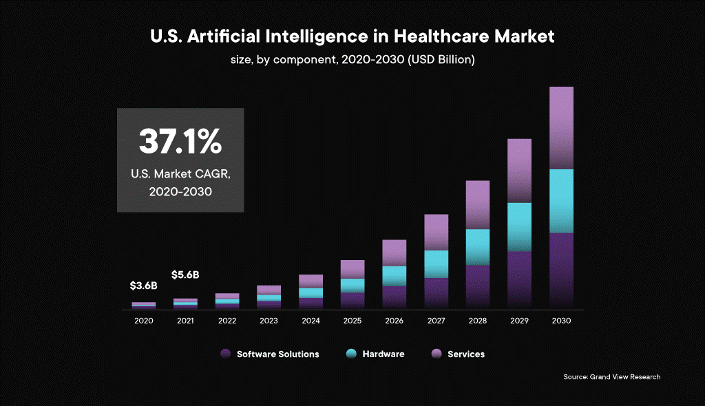
The global AI in healthcare will see a CAGR of 37.1% from 2022-2023!
So, it’s evident that AI in healthcare is brimming with potential. Here are some of the benefits of AI in healthcare:
Efficiency in clinical research, diagnosis, and treatment
Precision in advanced surgeries
Optimizing costs for healthcare organizations
Streamlining processes and administration for healthcare companies
Improving patient-doctor and patient-healthcare provider experiences
Contrary to popular opinion, using AI in healthcare will not replace humans but will make their lives easier. It will facilitate an optimal team effort scenario, streamlining the process and obtaining maximum efficiency, which is favorable for healthcare providers and patients.
Centralize Patient Information and Streamline Operations with AI in Healthcare
The accelerated shift towards the online ecosystem on all fronts is now a reality. It’s not just eCommerce businesses; even healthcare companies require an online presence nowadays to capitalize on patients. Healthcare providers use advanced medical devices, and with the current norm of connected technology, there is an inflow of an immense amount of data.
The Bigger Challenge?
While some organizations have solutions to manage data and generate patient information, the challenge lies in bringing structure to the data.
Healthcare organizations are left with a plethora of unstructured data, sometimes from multiple sources. Even top healthcare companies lack the proper means and solutions to manage data ranging from patient information and medical transcripts to medical records. Efficiently streamlining data from various information sources is a significant challengeandcannot be performed with relational databases.
The Universal Customer Data Platform is Affine’s AI solution for healthcare providers that combines multiple data sources and pools the information, creating a universal data lake.
Healthcare providers can leverage insights from this and create a universal patient profile that can be accessed worldwide. They can also personalize their efforts for customer reach and engagement more efficiently, owing to the centralized data ecosystem.
Ai In Healthcare to Optimize Costs And Increase Revenue
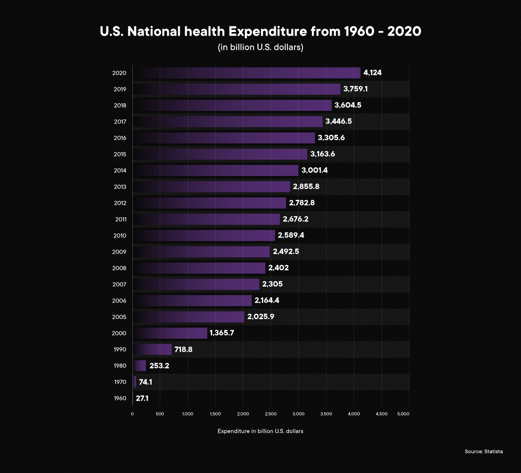
Healthcare prices stem from various factors. The United States is notorious for its ridiculously high healthcare costs, which spells a significant setback in terms of revenues for healthcare providers. The USA spent a whopping $4,124 Billion on healthcare in 2020! Modern-day inflation has made everything high-priced and expensive healthcare is a deterrent to many patients who ideally should take regular tests and visit practitioners. In the long run, this is an unsustainable model for healthcare companies.
Healthcare providers can create packages and plans that patients can subscribe to, ensuring business while providing value to patients both service and cost-wise for a sustainable operating model in the long run.
The Intelligent Pricing Solution is another Affine solution for healthcare providers that creates a uniform pricing model for patients. This smart solution only recommends required tests and procedures thanks to the patient information, thus making it possible for the companies to offer great prices while providing quality healthcare service.This is vital in developing a sustainable patient relationship while improving engagement and helps increase the ROI in the long run.
Use Of AI In Healthcare Is Essential for A Sustainable Future
The above solutions are just a glimpse of what AI is capable of for healthcare providers. According to this report, ML in the healthcare industry is estimated to generate a global value of over $100 Billion. In the future, we are looking at AI-powered predictive healthcare, where anomalies in human health and chronic diseases are identified with historical patient information, and preventive measures can be taken in advance to save lives.
People are embracing travel post the pandemic, and organizations are encouraging a work-from-anywhere culture. Healthcare needs a connected tech approach, and providers must opt for centralized AI solutions that can provide patient information oncommand. Not only does this make for an efficient, but it also improves the patient experience.
For healthcare providers, AI and ML-based solutions help engage and motivate patients, improve their lives, assist them in their day-to-day activities, and handle the inflow of customers smoothly.
This may sound quite simple, but we all witnessed what happened when COVID-19 hit the USA, and the healthcare system got choked handling the sheer number of patients. Despite having one of the most advanced healthcare systems in the world, the country was brought to its knees during the pandemic. When I mentioned earlier that AI assists humans and does not take over their jobs, I couldn’t find a better example than the healthcare industry. Healthcare employees are among most overworked, burnt out, and underrated.
AI in healthcare can aid organizations, patients, and healthcare employees at capacity and their absolute limit, helping them bypass various tasks.
What does Affine bring to the table?
Affine is a pioneer and a veteran in the data analytics industry and has worked with giants like BSN Medical, Optum, AIG, New York Life, and many other marquee organizations. From game analytics and media and entertainment to travel and tourism, Affine has been instrumental in the success stories of many Fortune 500 global organizations; and is an expert in personalization science with its prowess in AI & ML.
Learn more about how Affine can revamp your healthcare business!
As businesses take a global route to growth, two things happen. First, the complexity and unpredictability of business operations increase manifold. Second, organizations find themselves collecting more and more data – predicted to be up to 50% more by 2025. These trends have led businesses to look at Artificial Intelligence as a key contributor to business success.
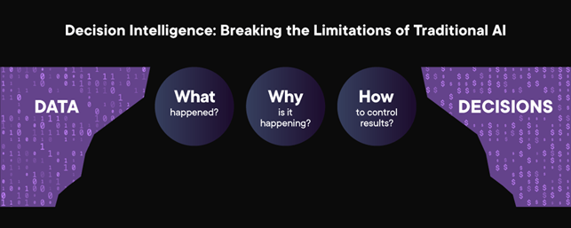
Despite investing in AI, top managers sometimes struggle to achieve a key benefit – enabling them to make critical and far-sighted decisions that will help their businesses grow. In an era of uncertainty, traditional models cannot capture unpredictable factors. But, by applying machine learning algorithms to decision-making processes, Decision Intelligence helps create strong decision-making models that are applicable to a large variety of business processes and functions.
The limitation of traditional AI models in delivering accurate decision-making results is that they are designed to fit the data that the business already has. This bottom-up process leads to data scientists concentrating more on data-related problems rather than focusing on business outcomes. Little wonder then that, despite an average of $75 million being spent by Fortune 500 companies on AI initiatives, just 26% of them are actually put into regular use.
Decision Intelligence models work on a contrarian approach to traditional ones. They operate with business outcomes in mind – not the data available. Decision Intelligence combines ML, AI, and Natural Language queries to make outcomes more comprehensive and effective. By adopting an outcome-based approach, prescriptive and descriptive solutions can be built that derive the most value from AI. When the entire decision-making process is driven by these Decision Intelligence models, the commercial benefits are realized by every part of the organization.
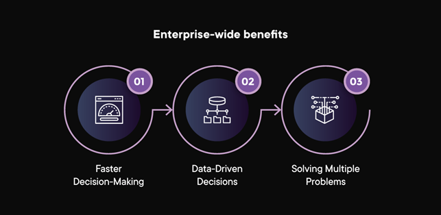
Incorporating Decision Intelligence into your operations delivers benefits that are felt by every part of your business. These benefits include:
Faster Decision-Making: Almost every decision has multiple stakeholders. By making all factors transparently available, all the concerned parties have access to all the available data and predicted outcomes, making decision-making quicker and more accurate.
Data-Driven Decisions Eliminate Biases: Every human process data differently. When misread, these biases can impact decisions and lead to false assumptions. Using Decision Intelligence models, outcomes can be predicted based on all the data that a business has, eliminating the chance of human error.
Solving Multiple Problems: Problems, as they say, never come in one. Similarly, decisions taken by one part of your operations have a cascading effect on other departments or markets. Decision Intelligence uses complex algorithms that highlight how decisions affect outcomes, giving you optimum choices that solve problems in a holistic, enterprise-wide way, keeping growth and objectives in mind.
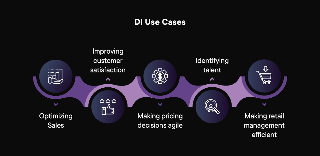
Decision Intelligence: One Technology, Many Use Cases
Decision Intelligence tools are effective across a multitude of business applications and industry sectors. Here are some examples of how various industries are using Decision Intelligence to power their growth strategies:
Optimizing Sales: Decision Intelligence can get the most out of your sales teams. By identifying data on prospects, markets, and potential risks, Decision Intelligence can help them focus on priority customers, predict sales trends, and enable them to forecast sales to a high degree of accuracy.
Improving customer satisfaction: Decision Intelligence-based recommendation engines use context to make customer purchases easier. By linking their purchases with historical data, these models can intuitively offer customers more choices and encourage them to purchase more per visit, thus increasing their lifetime value.
Making pricing decisions agile: Transaction-heavy industries need agility in pricing. Automated Decision Intelligence tools can predictively recognize trends and adjust pricing based on data thresholds to ensure that your business sells the most at the best price, maximizing its profitability.
Identifying talent: HR teams can benefit from Decision Intelligence at the hiring and evaluation stages by correlating skills, abilities, and experience with performance benchmarks. This, in turn, helps them make informed decisions with a high degree of transparency, maximising employee satisfaction and productivity.
Making retail management efficient: With multiple products, SKUs and regional peculiarities, retail operations are complex. Data Intelligence uses real-time information from stores to ensure that stocking and branding decisions can be made quickly and accurately.
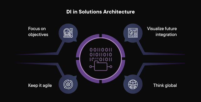
Incorporating Decision Intelligence into the Solutions Architecture
CTOs and solutions architects need to keep four critical things in mind when incorporating a Decision Intelligence into their existing infrastructure:
Focus on objectives: Forget the data available for a bit. Instead, finalize a business objective and stick to it. Visualize short sprints with end-user satisfaction in mind and see if the solution delivers the objective. This approach helps technical teams change their way of thinking to an objective-driven one.
Visualize future integration: By focusing on objectives, solution architects need to keep the solution open to the possibility of new data sets arising in the future. By keeping the solution simple and ready to integrate new data as it comes in, your Data Intelligence platform becomes future-proof and ready to deliver answers to any new business opportunity or problem that may come along.
Keep it agile: As a follow-up to the above point, the solution needs to have flexibility built in. As business needs change, the solution should be open enough to accommodate them. This needs flexible models with as few fixed rules as possible.
Think global: Decision Intelligence doesn’t work in silos. Any effective Decision Intelligence model should factor in the ripple effect that a decision – macro or micro – has on your entire enterprise. By tracking dependencies, the solution should be able to learn and adapt to new circumstances arising anywhere where your business operates.
Machine learning and artificial intelligence are niche technologies, and companies have started thinking about or utilizing these technologies aggressively as part of their digital transformation journey. These advancements have changed the demand curve for data scientists, machine learning, and artificial intelligence technologists. Artificial intelligence-driven digital solutions require cross-collaboration between engineers, architects, and data scientists, and this is where a new framework, “AI for you, me, and everyone,” has been introduced.
To Sum Up
Decision Intelligence is a powerful means for modern businesses to take their Artificial Intelligence journey to the next level. When used judiciously, it helps you make accurate, future-proof decisions and maximize customer and employee satisfaction, letting you achieve your business objectives with the least margin of error.
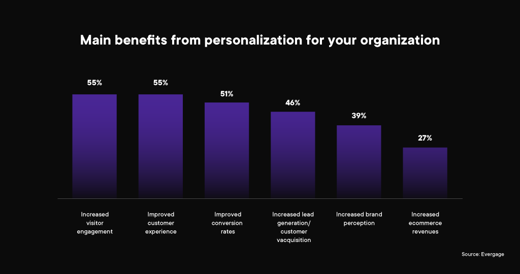
Exceptional customer experience through personalization is the elixir of online shopping. 95% of companies increased their ROI by 3X with personalization efforts. There is always the debate about privacy and handling of data, but the younger next-generation of shoppers are open to it, and the future is set to see data-backed hyper-personalization across multiple touch points in E-Commerce platforms, in my opinion.
The challenge for E-Commerce businesses with personalization is multifold. Customers seek a device-agnostic experience in online shopping, so a uniform shopping experience is a basic need. On top of that, there is a plethora of data inflow, which makes for great potential but only if it is leveraged aptly by E-Commerce businesses. With the prowess of AI, the possibilities are many and colorful for E-Commerce businesses.
There is an immediate need for a centralized solution, considering the omnichannel nature of shopping amongst online customers. With data inflow from various sources, the alternative is just a large amount of unstructured pile of data that does not provide value for the business.
This is where AI will rewrite the rules and set the foundation for a new type of unparalleled customer experience in E-Commerce.
Data & AI-2 sides of the personalization coin for E-Commerce
Personal opinion -I’m willing to share data for a no-nonsense experience on the internet. Eventually, with connected tech and synced accounts becoming a norm by the day, online shoppers will opt for the same, considering the benefits. In my opinion, we’re too co-dependent on the internet for our day-to-day activities and sharing data for a better shopping experience is a valid tradeoff.
3d product previews & virtual try-on are the tips of the iceberg of what AI has in store to revolutionize the customer experience and write the future for E-Commerce companies.
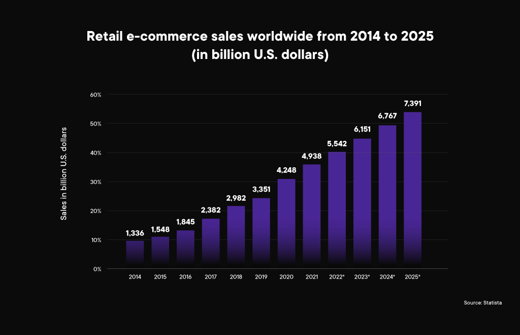
AI in movies is mostly dystopian, about rogue software taking over the world, but in the real world, there is a drastic contrast to the applications and potentials of AI in day-to-day use cases. AI isn’t anymore a niche tech reserved for a few organizations.The infusion of technology in E-Commerce has made life easier for people, and the data shows. Just take a look at the worldwide sales, the growth is unprecedented and projected to spike through the roof in the coming years.
So, naturally, as someone working in close quarters with AI experts and E-Commerce veterans, I couldn’t help but speculate about the future of the marriage between the two.
Next level personalization for exceptional user experience
I remember the good old days of AOL messenger, Yahoo-Mail & My-Space. The internet at its cusp was pure, and people just hung out and wondered at the marvel of this infant tech and its dynamic capability.
With great power comes great responsibilities, and the internet opened the gateway to access various types of data; this, paired with the eventual shift towards online shopping, would work wonders for businesses. This was inevitable as the monetization of the internet was bound to happen. When anything is free, you’re the product.
I’m spoiled by the Apple ecosystem and can’t get enough of the seamless interaction and experience when I use any device, be it my laptop, mobile, or iPad. Imagine this for E-Commerce businesses on a gigantic scale.
For E-commerce companies, AI technologies can vastly improve product selection and overall user experience, which becomes a crucial part of the customer lifecycle.
Big data offers a plethora of opportunities for E-commerce personalization. Segmenting and customizing the experience is made possible by analyzing historical data. Even the messaging is personalized to the core, ensuring the relevancy factor is preserved.
Affine’s AI-powered Hyper Personalized Marketing Experience is one such solution that leverages customer behavior data, segmentation data, and cohort analysis at scale
What do customers gain from this?
As an avid online shopper, I appreciate the personalized shopping experience on an E-Commerce platform. Getting to see the products with utmost relevance is a positive shopping experience rather than being spammed with random recommendations; at least, that has been my experience so far.
When E-Commerce businesses leverage data properly, it creates an exceptional shopping and customer experience and results in return customers. We all have our favorite shopping websites, and personalization has played a crucial role in them.
What do E-Commerce businesses gain from this?
First things first: – a centralized workhorse robust personalization ecosystem,minimal data leak, and making sense of every customer move and converting it into a quality-of-life add-on with personalization, targeting, and segmentation.
Such a sophisticated solution makes it possible to identify the most feasible customers and target them with hyper-personalized efforts. The data is the only limitation to the possibilities here. Not only does this net the best possible customers for the business, but it optimizes the marketing efforts making the whole targeting process efficient. Ad budgets are kept in check while ensuring superior ad display and performance.
I’ve spent fat budgets on marketing only to receive lukewarm prospects. I’ve also spent conservatively with proper data-powered personalized marketing initiatives that have resulted in excellent conversions. Centralized AI solutions provide complete accountability for marketing spend, helping E-Commerce businesses measure every dollar spent per lead.
Automation is seamless with AI
Contrary to popular opinion, AI is not about taking over human jobs; it is more about making our lives easier. Customer support is one of the most tasking efforts in the E-Commerce business. I’ve had my fair share of endless calls with customer support with language and technical issues. I know you’ve all been a part of at least one such instance in your lifetime.
The potential for customer support automation via chatbots is a fast-tracking of the entire process and is already seen with giants like Amazon.
E-Commerce businesses, small or large, can leverage AI to automate mundane tasks and basically run your online store to an extent without human intervention and take care of the overall processes in their day-to-day activities.
Be it automating marketing efforts, support, customer engagement, or advertising, AI has the clout to not only handle but also excel in outperforming manual labor while casually being time and cost-efficient in the process. Automating the marketing process also brings up a 451% increase in qualified leads.
Combat fraud activities with AI’s security prowess
We’ve all known of someone who has fallen prey to online fraud and I know I do. With the convenience of seamless transactions, there is also the vulnerability of fraud in E-Commerce transactions. A research shows that online payment fraud could lead to a global merchant loss of up to $343 billion from 2023 to 2027.
Despite security measures, these instances call for drastic innovations in verification tools and authentication processes. AI and ML algorithms are the only effective option to combat online threats at such a higher scale in the count of millions of transactions, with predictive analytics to detect behavioral patterns and suspect behavior resulting in fraudulent transactions.
Brand loyalty, repeat business, and ROI
A gazillion data points are analyzed so that customers can get the best shopping experience and keep coming back for more. Sure, but E-Commerce businesses have the most to leverage from intelligent AI algorithms running through a plethora of data points. As I mentioned earlier, the possibilities are immense and lucrative.
I have my go-to sites for shopping, and I have valid reasons for that. So do customers, hence the need for AI in E-Commerce platforms. Personalization may make it sound like the customer is reaping all the benefits, but that’s the intention.
The spend more get more is outdated, and efficiency is the need of the hour. Inefficient business operations cause a major dent in business revenues
Conclusion
The era of big data is here. Digital dominance is set to take over the world, and E-Commerce sites are more or less the new convenience stores in the digital age. I see a lot of competition; I see a lot of potential.
75% of businesses already use AI and are on the right track in the long run. Having run a startup myself, I understand the qualms about the cost of implementing AI. But the big picture justifies it and how.
AI in E-Commerce is not even a novelty anymore; it is a must-have. An online E-Commerce is a global marketplace, and the standards are already set. It’s excel or be expelled. A proper flow to guide your customers through their buying experience is the basic requirement to sustain and perform in the long run.
What does Affine bring to the table?
Affine is a pioneer and a veteran in the data analytics industry and has worked with giants like Warner Bros Theatricals, Zee 5, Disney Studios, Sony, Epic, and many other marquee organizations. From game analytics and media and entertainment to travel & tourism, Affine has been instrumental in the success stories of many Fortune 500 global organizations; and is an expert in personalization science with its prowess in AI & ML.
Learn more about how Affine can revamp your E-Commerce business!
Human Activity Recognition using high-dimensional visual streams has been gaining popularity in recent times. Using a video input to categorize human activity is primarily applied in surveillance of different kinds. At hospitals and nursing homes, this can be used to immediately alert caretakers when any of the residents are displaying any sign of sickness – clutching their chest, falling, vomiting, etc. At public places like airports, railway stations, bus stations, malls or even in your neighborhoods, the activity recognition becomes the means to alert authorities on recognizing suspicious behavior. This AI solution is even useful for identifying flaws in and improving the form of athletes and professionals ensuring improved performance and better training.
Why Use Multimodal Learning for Activity Recognition?
Our experience of the world is multimodal in nature, as quoted by Baltrušaitis et al. There are multiple modalities a human is blessed with. We can touch, see, smell, hear, and taste, and understand the world around us in a better way. Most parents would remember their kid’s understanding of “what a dog is” keeps improving after seeing actual dogs, videos of dogs, photographs of dogs and cartoon dogs and being told that they are all dogs. Just seeing a single video of an actual dog does not help the kid identify the character “Goofy” as a dog. It is the same for machines. Multimodal machine learning models can process and relate the information from multiple modalities, learning in a more holistic way.
This blog serves as the captain’s log on how we combined the effectiveness of two modalities – Static Images and Videos – to improve the classification of human activities from videos. Algorithms for video activity recognition are based on dealing with only spatial information (images), or both spatial and temporal information (videos). Algorithms were used for both static images and videos for the activity recognition modeling. Fusing both models together made the resultant multimodal model far better than each of the individual unimodal models.
Multimodal Learning for Human Activity Recognition – Our Recipe
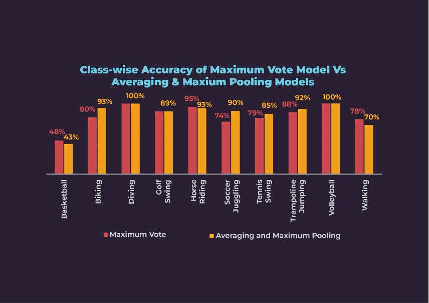
Our goal was to recognize 10 activities – basketball, biking, diving, golf swing, horse riding, soccer juggling, tennis swing, trampoline jumping, volleyball spiking, and walking. We created the multimodal models for activity recognition by fusing the two unimodal models – image-based and video-based – using the ensemble method, thus enhancing the effect of the classifier.
There are different methodologies for Multimodal learning as is described by Song et al., 2016, Tzirakis et al., 2017, and Yoon et al., 2018. One of the techniques is ensemble learning, in which 2DCNN model and 3DCNN models are trained separately and the final softmax probabilities are combined to get predictions. Other techniques include joint representation, coordinated representation etc. A detailed overview is available in Baltrušaitis et al., 2018.
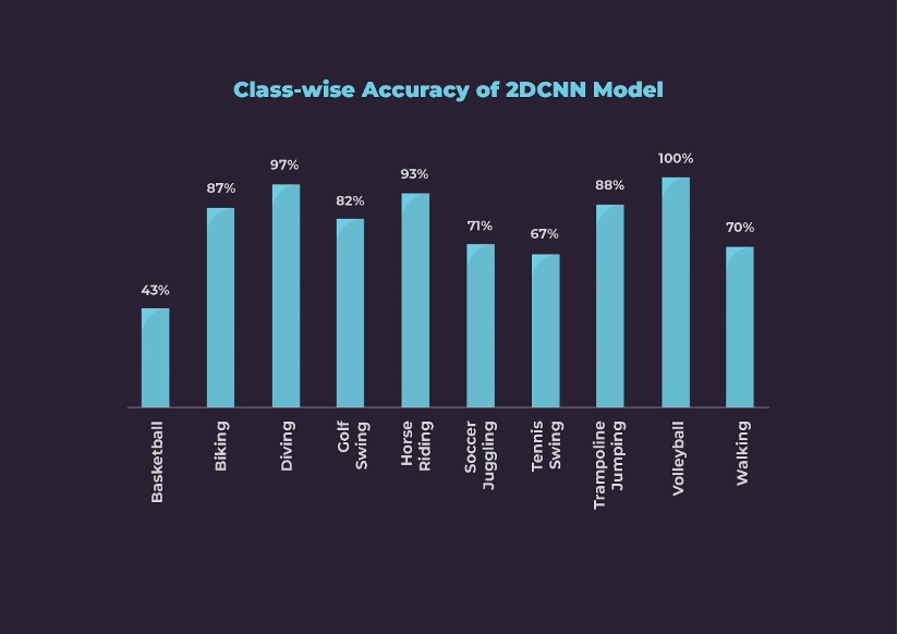
The First Modality – Images: We trained a 2DCNN model with VGG-16 architecture and equipped our model with batch normalization and other regularization methods, since the enormous number of frames
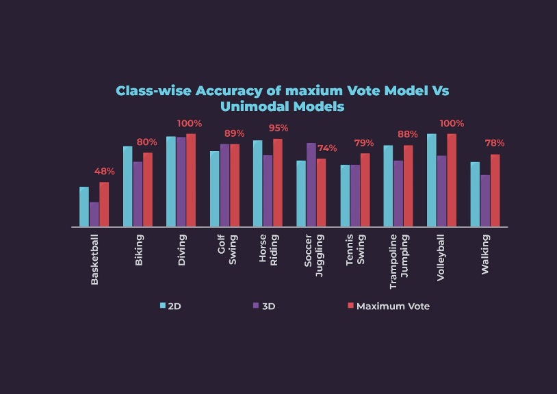
caused overfitting. We observed that deeper architectures were less accurate. We achieved 81% clip-wise accuracy. However, the accuracies are very poor on some classes such as basketball, soccer juggling, tennis, and walking as can be seen below.
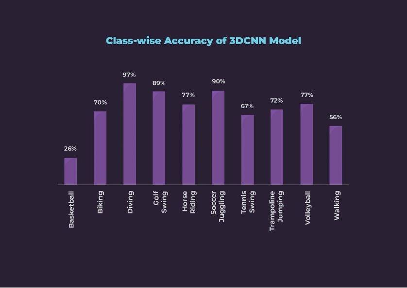
Second Modality –Videos: The second model was trained with 3DCNN architecture, which took 16 frames as one chunk called as a block. We incorporated various augmentations, batch normalization, and regularization methods. During the exercise, we observed that 3D architecture is sensitive to the learning rate. In the end, we achieved a clip-wise accuracy of 73%. Looking at the accuracies for individual classes, this model is not the best, but it is much better than the 2DCNN for Soccer Juggling and Golf classes. Class-wise accuracies can be seen below.
Our next objective was to ensure that the learnings from both modalities are combined to create a more accurate and robust model.
Our Secret Sauce for Multimodal learning – The Ensemble Method
For fusing the two modalities, we resorted to ensemble methods (Zhao, 2019). We experimented with two ensemble methods for the Multimodal learning:
1. Maximum Vote – Mode from the predictions of both models is taken as the predicted label.
2. Averaging and Maximum Pooling – Weighted sum of probabilities of both models is calculated to decide the predicted label.
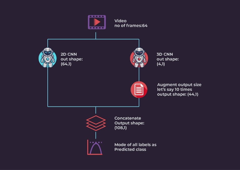
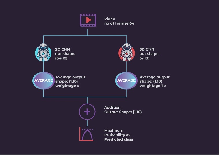
Maximum Vote Ensemble Approach: Let us consider a video consisting of 64 frames. We fed these frames to both 2D and 3D models. The 2D model produced an output for each frame resulting in 64 tensors with a predicted label. Similarly, the 3D model produced a label for 16 frames, thus finally generating 4 tensors for 64 frames video. To balance the weightage of the 3D model, we augment the output tensors of the 3D model by repeating the tensor multiple times. Finally, we concatenated the output tensors from both models, and selected the modal class (the class label with the highest occurrence) as the prediction label.
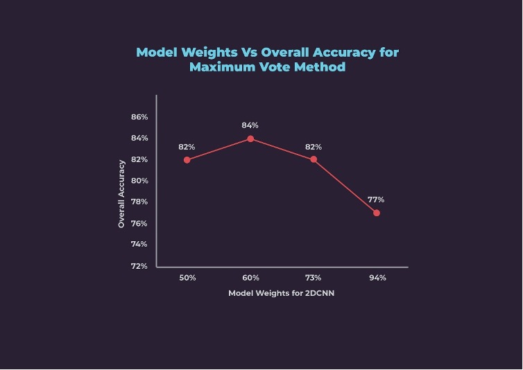
We iteratively experimented with different weightages for both models and checked the corresponding overall accuracy as shown below. Maximum overall accuracy of 84% was achieved at 60% weightage to the 2D model and 40% weightage to the 3D model.
At 60:40 weightage for 2D:3D, the Maximum Vote ensemble method has performed better than either of the unimodal models except for Biking and Soccer Juggling.
Averaging and Maximum Pooling Ensemble Method: Consider that we are feeding a video with 64 frames to both models, the 2D model which generates 64 tensors with probabilities for every class and the 3D model will generate 4 tensors with probabilities for each of 10 classes. We calculate the average of all 64 tensors from the 2D model to get the average probability for every class. Similarly, we calculate the average of the 4 tensors from the 3D model. Finally, we take the weighted sum of resulting tensors from both models. We select the class with maximum probability as the predicted class.
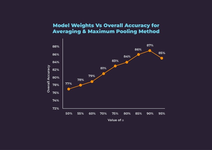
The equation for the weight in Averaging and Maximum Pooling method is:
Multimodal = α*(2D Model) + (1-α)*(3D Model)
We experimented with different values of α and compared the resulting overall accuracies as shown below. With equal weightage to both models, we achieved 77% accuracy. With the increase in α, i.e., weightage to 2D model, multimodal accuracy increased. We achieved the best accuracy of 87% at 90% weightage to the 2D model and 10% weightage of the 3D model.
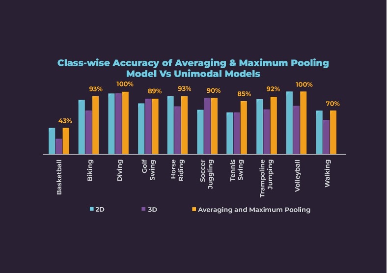
The class-wise accuracy for the Averaging and Maximum Pooling method is low for Basketball and Walking classes. However, the class-wise accuracies are better than or at least the same as the unimodal models. The accuracies for Soccer Juggling and Tennis Swing improved the most from 71% and 67% for the 2D model to 90% and 85% respectively.
Conclusion
Beyond doubt, our Multimodal models performed better than the Unimodal ones. Comparing the multimodal engines, Averaging and Maximum Pooling performed better than the Maximum Vote method, as is evident from the overall accuracies of 87% and 84% respectively. The reason is that the Averaging and Maximum Pooling method considers the confidence of the predicted label whereas, the Maximum Vote method considers only the label with maximum probability.
In Human Activity Recognition, we believe the multimodal learning approach can be improved further by incorporating other modalities as well. Such as Facebook’s Detectron model or pose estimation method.
Our next plan of action is to explore more forms of multimodal learning for activity recognition. Using features addition/ layers are fusing features can be effective in learning features better. Another way of proceeding would be to add different modalities like pose detection feed, motion detection feed and object detection feed to provide better results. No matter the approach, fusing modalities has a corresponding cost factor associated with it. While we have 40.4 million trainable parameters in the 2DCNN model and 78 million parameters in the 3DCNN models, the multimodal model has 118.5 million parameters to train on. But this is a small amount to pay considering the limitless applications that can be made viable because of the performance improvement provided by the multimodal models.
I believe you have gone through part 1 and understood what Attribution and Incrementality mean and why it is important to measure these metrics. Below, we will discuss some methods that are commonly used across the industry to achieve our goals.
Before we dive into the methods, let us understand the term Randomised Controlled Trials (RCT). And by the way, in common jargon, they are popularly known as A/B tests.
What are Randomized Controlled Trials (RCT)?
Simply put, it is an experiment that measures our hypothesis. Suppose we believe (hypothesis) that the new email creative (experiment) will perform (measure) better than the old email creative. Now, we will randomly split our audience into 2 groups. One of them, the control group, keeps receiving the old emails, and the other, the test group, keeps receiving the new email creative.
Now how do you quantify your measure? How do you understand your experiment is performing better? Choose any metric that you think should determine the success of the new email creatives. Say, Click-through Rate (CTR). Thus, if the test group has a better CTR than the control group, you can say that the new email creative is performing better than the old email creative.
Some popular methods to run experiments:
Method 1:
User-Level Analysis
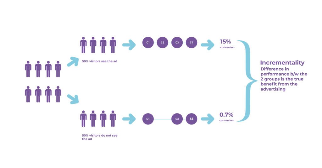
Illustration for Incrementality
One of the simple ways to quantify incrementality would be to run an experiment as done in the diagram. Divide your sample into two random groups. Expose the groups to a different treatment; for example, one group receives a particular email/ad, and the other does not.
The difference in the groups reflects the true measurement of the treatment. This helps us quantify the impact of sending an email or showing a particular ad.
Method 2:
Pre/Post Analysis
This is an experiment that can be used to measure the effect of a certain event or action by taking a measurement before (pre) and after (post) the start of the experiment.
You can introduce a new email campaign during the test period and measure the impact over time of any metric of your interest by comparing it against the time when the new email campaign was not introduced.
Thus, by analyzing the difference in the impact of the metric you can estimate the effect of your experiment.
Things to keep in mind while performing pre/post analysis:
Keep the control period long enough to get significant data points
Keep in mind that there might be spillover in results during the test phase, so we should ensure that the impact of this spillover is not missed
Ensure that you keep enough time for the disruption period. It refers to the transient time just after you have launched the experiment
It is ideal to avoid peak seasons or other high volatility periods in the business for these experiments to yield conclusive results
Method 3:
Natural Experiment
It is similar to the A/B test, where you can observe the effect of a treatment (event, feature) on different samples but not having the ability to define/control the sample. So, it is similar to Randomised Controlled Trial, but you cannot control the environment of the experiment.
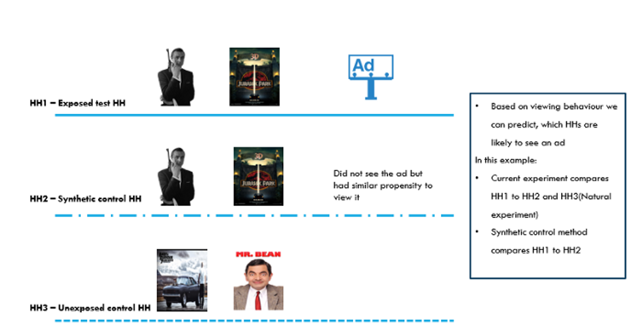
Suppose you want to understand the impact of a certain advertisement. If you do what we have explained above in Method 1, and create 2 groups, a control group that is not shown the particular advertisement and a test group that has been shown the ad and try to measure the impact of the advertisement, you might make a basic mistake. The groups may not be homogenous to start with. The behavior of the groups can be different from the start itself, so you are expected to see very different results and thus cannot be sure of the effectiveness of the ad.
We need to decrease the bias by attempting resampling and reweighting techniques. To tackle this, we can create Synthetic Control Groups(SCGs).
Find below an example with an illustration for the scenario:
We will create SCGs within the unexposed groups. We will try to understand which households (HHs) missed an ad, but based on their viewing habits are similar to those households (HHs) which have seen one.
Images:
James Bond: This Photo by Unknown Author is licensed under CC BY-NC;
Jurrasic park: This Photo by Unknown Author is licensed under CC BY-NC-ND;
Fast and Furious: This Photo by Unknown Author is licensed under CC BY-NC-ND;
Mr Bean: This Photo by Unknown Author is licensed under CC BY-NC
Another sub-method that is out of the scope for this blog is to attach a weight to every household based on their demographics attributes(gender, age, income, etc) using iterative proportional fitting and the comparison happens on the weighted results.
Method 4:
Geo Measurement
Geo measurement is a method that utilizes the ability to spend and/or market in one geographic area (hence “geo”) vs. another. A typical experiment consists of advertising in one geo (the “on” geo) and holding out another geo (the “off” geo), and then measuring the difference between them i.e., the incrementality caused by the treatment. One also needs to account for pre-test differences between on and off geographies either by normalizing these before evaluation or adjusting for this post-hoc analysis.
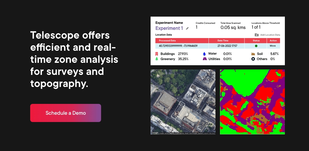
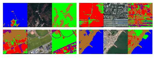
Satellite image segmentation has been in practice for the past few years, and it has a wide range of real-world applications like monitoring deforestation, urbanization, traffic, identification of natural resources, urban planning, etc. We all know that image segmentation is the process of color coding each pixel of the image into either one of the training classes. Satellite image segmentation is the same as image segmentation. In this process, we use landscape images taken from satellites and perform segmentation on them. Typical training classes include vegetation, land, buildings, roads, cars, water bodies, etc. Many Convolution Neural Network (CNN) models have shown decent accuracy in satellite image segmentation. One of these models, which is a highlight, is the U-Net model. Though the U-Net model gives decent accuracy, it still has some drawbacks like predicting classes with very near-distinguishable features, being unable to predict precise boundaries, and so on. In order to address these drawbacks, we have performed satellite image segmentation using the Basic FPN + PointRend model from the Detectron2 library, which has significantly rectified the drawbacks mentioned above and showed a 15% increase in accuracy when compared to the U-Net model on the validation dataset used.
In this blog, we will start by describing the objective of our experiment, the dataset we used, a clear explanation of the FPN + PointRend model architecture, and then demonstrate predictions from both U-Net and Detectron 2 models for comparison.
Objective
The main objective of this task is to perform semantic segmentation on satellite images to segment each image’s pixels into either of the five classes considered: greenery, soil, water, building, or utility. Constraints are anything related to plants and trees like forests, fields, bushes, etc., considered single-class greenery. Same for soil, water, building, and utility (roads, vehicles, parking lots, etc.) classes.
Data Preparation for Modeling
We have created 500 random RGB satellite images using the Google Maps API for modeling. For segmentation tasks, we need to prepare annotated images in the format of RGB masked images with height and width the same as the input image and each pixel value corresponds to the respective class color code (i.e., greenery – [0,255,0], soil – [255,255,0], water – [0,0,255], buildings – [255,0,0], utility – [255,0,255]). For the annotation process, we chose the LabelMe tool. Additionally, we have performed image augmentations like horizontal flip, random crop, and brightness alterations on images to let the model robustly learn the features. After annotations are done, we made a train and validation split for the dataset in the ratio of 90:10. Below is a sample image from the training dataset and the corresponding RGB masked image.
Fig 1: A sample image with a corresponding annotated RGB mask from the training dataset
Model Understanding
For modeling, we have used the Basic FPN segmentation model + PointRend model from Facebook’s Detectron2 library. Now let us understand the architecture of both models.
Basic FPN Model
FPN (Feature Pyramid Network) mainly consists of two parts: encoder and decoder. An image is processed into a final output by passing through the encoder first, then through the decoder, and finally through a segmentation head for generating pixel-wise class probabilities. In the bottom-up encoder, the approach is performed using the ResNet encoder, and in the decoder, the top-down approach is performed using an adequately structured CNN network.
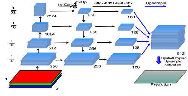
In the bottom-up approach, the RGB image is passed as input, and then it is processed through all the convolution layers. After passing through each layer, the output of that particular layer is sent as input to the next layer as well as input to the corresponding convolution layer in the top-down path, as seen in fig 2. In the bottom-up approach, image resolution is reduced by 1/4th the input resolution of that layer as we go up, therefore, performing down sampling on the input image.
In the top-down path for each layer, input comes from the above layer and from the corresponding bottom-up path layer, as seen in fig 2. These two inputs are merged and then sent to the layer for processing. Before merging to equate the channels of both input vectors, the input from the bottom-up path is passed through a 1*1 convolution layer, which results in an output of 256 channels, and the input from the above top-down layer is upsampled 2 times using the nearest neighbor’s interpolation method. Then both the vectors are added and sent as input to the top-down layer. The output of the top-down layer is passed 2 times successively through the 3*3 convolution layer, which results in a feature pyramid with 128 channels. This process is continued till the last layer in the top-down path. Therefore, the output of each layer in the top-down path is a feature pyramid.
Each feature map is upsampled such that its resulting resolution is the same as 1/4th of the input RGB image. Once upsampling is done, they are added and sent as input to the segmentation head, where 3*3 convolution, batch normalization, and ReLU activation are performed. To reduce the number of channels in the output to the same as the number of classes, we apply 1*1 convolution. Then spatial dropout and bi-linear interpolation upsampling are performed to get the prediction vector with the same resolution same as the input image.
Technically, in the FPN network, the segmentation predictions are performed on a feature map that has a resolution of 1/4th of the input image. Due to this, we must compromise on the accuracy of boundary predictions. To address this issue, PointRend model is used.
PointRend Model
The basic idea of the PointRend model is to see segmentation tasks as computer graphics rendering. Same as in rendering where pixels with high variance are refined by subdivision and adaptive sampling techniques, the PointRend model also considers the most uncertain pixels in semantic segmentation output, upsamples7t them, and makes point-wise predictions which result in more refined predictions. The PointRend model performs two main tasks to generate final predictions. These tasks are,
Points Selection – how uncertain points are selected during inference and training
Point-Wise Predictions – how predictions are made for these selected uncertain points
Points Selection Strategy
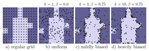
During inference, random points are selected where the probabilities in the coarse prediction output (prediction vector which has a resolution equal to 1/4th of the input image) from the FPN model have class probabilities near to 1/no. of the classes, i.e., 0.2 in our case as we have 5 classes. But during training, instead of selecting points only based on probabilities first, it selects kN random points from a uniform distribution. Then it selects βN most uncertain points (points with low probabilities) from among these kN points. Finally, the remaining (1 – β)N are sampled from a uniform distribution. For the segmentation task during training, k=3 and β=0.75 have shown good results. See fig 3 for more details on the point selection strategy during training.
Fig 3: Point selection strategy demonstration (Image source [2])
Point-Wise Predictions
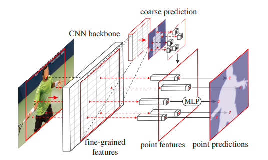
Point-wise predictions are made by combining two feature vectors:
Fine-Grained Features – At each selected point, a feature vector is extracted from the CNN feature maps. The feature vector can be extracted from a single feature map of res2 or multiple feature maps, e.g., res2 to res5 or feature pyramids.
Coarse Prediction Features – Feature maps are usually generated at low resolutions. Due to this fine feature, information is lost. For this, instead of relying completely on feature maps, course prediction output from FPN is also used in the extracted feature vector at selected points.
The combined feature vector is passed through MLP (multi-layer perceptron) head to get predictions. The MLP has a weight vector for each point, and these get updated during training by calculating loss similar to the FPN model, which is categorical cross-entropy.
Combined Model (FPN + PointRend) Flow
Now that we understand the main tasks of the PointRend model, let’s understand the flow of the complete task.
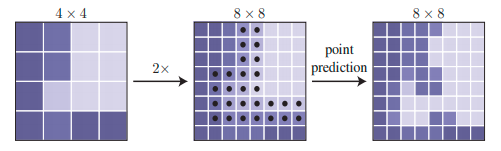
First, the input image is sent to the CNN network (in our case, the FPN model) to get a coarse prediction output (in our case, a vector of ¼th the resolution of the input image with 5 channels). This coarse prediction vector is sent as input to the PointRend model, where it is upsampled 2* times using bilinear interpolation, and N uncertain points are generated using the PointRend point selection strategy. Then, at these points, new predictions are made using a point-wise prediction strategy with a MLP head (multi-layer perceptron), and this process is continued till we reach the desired output resolution. Suppose the course prediction output resolution is 7*7 and the desired output resolution is 224*224; the PointRend upsampling is done 5 times. In our case, the input resolution is ¼th of the desired output resolution. Therefore, PointRend upsampling is performed twice. Refer to fig. 4 and 5 for a better understanding of the flow.
Fig 4: PointRend model process flow (Image source [2])
Fig 5: PointRend model up sampling and point-wise prediction demo for 4*4 course prediction vector (Image source [2])
Results
For model training, we have used Facebook’s Detectron2 library. The training was done using an Nvidia Titan XP GPU with 12GB of VRAM and performed for 1 lakh steps with an initial learning rate of 0.00025. The best validation IoU was obtained at the 30000th step. The accuracy of Detectron2 FPN + PointRend outperformed the UNet model for all classes. Below are some of the predictions from both models. As you can see Detectron2 model was able to distinguish features of greenery and water class when U-Net failed in almost all cases. Even the boundary predictions of the Detectron2 model are far better than U-Net’s.
Fig 6: Sample predictions from UNet and Detectron2 model. Per image left is the prediction from UNet model, the middle is original RGB image and right is the prediction from Detectron2 model
Takeaway
In this blog, we have understood how the Detectron 2 FPN + PointRend model performs segmentation on the input image. The PointRend model can be applied as an extension to any image segmentation tasks to get better predictions at class boundaries. As further steps to improve accuracy, we can increase the training dataset, do augmentations on images, and play with hyperparameters like learning rate, decay, thresholds, etc.
Most of our readers who work with Machine Learning or Deep Learning models daily understand the struggle of peeking at the terminal to check for the completion status of the model training. Models training for hundreds of epochs can take several hours to complete. When you train a deep learning model on Google Colab, you’ll want to know your training progress to proceed further.
The saying, “A watched pot never boils faster,” seems to be relevant in the case of Machine learning or Deep Learning Model Training. Hyper Dash could be a helpful tool for all those situations.
Hyper Dash can monitor model training remotely on i0S, Android, or web URL. You can check the progress, stay informed about significant training changes, and get notified once your training is complete.
You can simultaneously monitor all your models running on different GPUs or TPUs and arrive at the best result. It maintains a log for results and hyper-parameters used, notifying you of the best one completed.
The Hyper Dash Convenience:
It is fast and user friendly.
Tracks hyper-parameters of the experiments and different functions.
Stores Graph performance metrics in real time · It can be viewed remotely on the Web, iOS, and Android without self-hosting (e.g., Tensorboard).
It saves the print output of the user’s experiment (standard out / error) as a local log file.
It notifies the user when a long-running experiment is completed.
Implementing Hyper Dash:
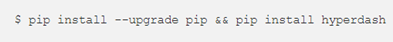
Installations on terminal/jupyter notebook.
It’s an easy to install PyPI package in the python module.
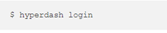
Next, you have to sign up for the hyper dash account
You can sign-up via mail or GitHub account. And when you log in, you will see the message above on your terminal/jupyter notebook.
Installation on phone.
Download the mobile application on your phone using Google Play/App store.
Once you have signed in, you can access experiments and their results on your phone.
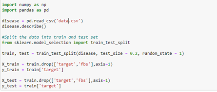
Implementing real-time tracking for modeling experiments.
First we import the required libraries. Then we import the dataset to be read, and split them for training and testing. After this, we add the target columns as y_train and y_test and drop the target variables from them.
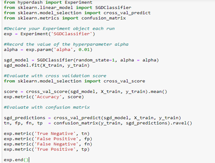
Now, we import the hyper dash library and its required modules. And after that, we define each experiment with an experiment name shown on your phone to identify your experiment uniquely.
We fit the model and test it on the test data set as hygiene. We can also view the confusion matrix of the entire model on our phone once the training is completed. We must add a method called exp.metric() to define our parameters like False Positives, False Negatives, True Positives, and True Negatives of our experiment.
Steps to use Hyperdash application are as follows-
Name: It declares the experiment object in each run with the Experiment(name).
Parameters: It records the value of any hyper-parameter with exp.param(‘name’, value) of the model.
Metrics: It records the value of any metric we wish to see with exp.metric(‘name’, score).
End: It marks the end of the experiment with exp.end().
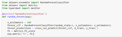
An added decorator experiment:
The above experiment will never close without an exp.end() command as it marks the end of the experiment. To avoid this confusion, we can always wrap our entire experiment command in a decorator as follows-
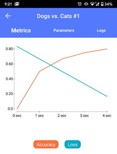
So once you start the modeling, you can track the experiment in real time on your phone.
Take for instance the following below:
These are experiments from different GPUs. You can select any model to observe the total time taken to run the model. Additionally, you get notified as soon as you complete the model training.
We can see different parameters and logs for every experiment. There is also a chart of confusion matrices with several parameters.
Conclusion
Hyper Dash is a user friendly application to track your model trainings. You can use the app with Tensorflow, Pytorch, etc. with compatibility across platforms and notification features for your phone.
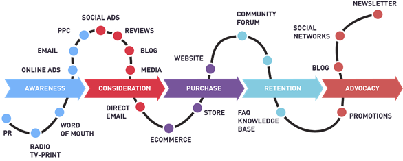
Suppose you are looking for a product on a particular website. As soon as you commence on the journey of making; the first search for a product, fidgeting on the idea to either buy it or not, and finally purchasing it, you are targeted or tempted by various marketing strategies through; various channels to buy the product.
You may start seeing the ads for the particular product on social media websites, on the side of various web pages, receive promotional emails, etc. This entire experience through these different channels that you interact with; will be referred to as touchpoints.
So, to sum up, whenever you provide an interest/signal to a platform that you are going to purchase a certain product, you may interact with these touchpoints mentioned above.
The job of a marketing team of a particular company is to utilize the marketing budget in a way that they get the maximum return on the marketing spend, i.e. to ensure that you buy their product.
So to achieve this, the marketing team uses a technique called Attribution.
What is Attribution?
Attribution is also known as Multi-Touch Attribution. Moreover, it’s an identification that walks you through of a set of user actions/events/touchpoints that drive a certain outcome or result and the assignment of value to each of those events/touchpoints.
Why is Attribution Important?
The main aim of marketing attribution is to quantify the influence of various touchpoints on the desired outcome and optimize their contribution to the user journey to maximize the return on marketing spend.
How does Attribution Work?
Assume; you had shown an interest in buying sneakers on Amazon. You receive the email tempting you to make the purchase, and finally, after some deliberation, you click on it and make the purchase. In a simple scenario, the marketing team will attribute your purchase to this email, i.e. they will feel that the email channel is what caused the purchase. They will think that there is a causal relationship between the targeted email and the purchase decision.
Suppose this occurrence is replicated across tens of thousands of users. The marketing team feels that email has the best conversion when compared to other channels. They start allocating more budget to it. They spend money on aesthetic email creatives, hire better designers, send more emails as they feel email is the primary driver.
But, after a month, you notice that the conversion is reducing. People are not interacting with the email. Alas! The marketing team has wasted the budget on a channel that they thought was causing the purchases.
Where did the Marketing Team go Wrong?
Attribution models are not causal, signifying that they give the credit of a transaction to a channel that may not necessarily cause that transaction. So, it was not only the emails that were causing the transactions; but there might have been another important touchpoint/touchpoints that were actually driving the purchase.
Understanding Causal Inference
The main goal of the marketing team is to use the attribution model to infer causality, and as we have discussed, they are not necessarily doing so. We need Causal Inference to truly understand the process of cause and effect of our marketing channels. Causal Inference deals with the counterfactual; it is imaginative and retrospective. Causal inference will instead help us understand what would have happened in the absence of a marketing channel.
Ta-Da!! Enters Incrementality. (Incrementality waiting the entire time to make its entrance in the blog)
What is Incrementality?
Incrementality is the process of identifying an interaction that caused a customer to do a certain transaction.
In fact, it finds the interaction that, in its absence, a transaction would not have occurred. Therefore, incrementality is the art of finding causal relationships in the data.
It is tricky to quantify the inherent relationships among touchpoints, so I have dedicated part 2 to discuss various strategies that are used to measure incrementality and how a marketing team can better distribute its budget across marketing channels.
Natural Language Inferencing (NLI) task is one of the most important subsets of Natural Language Processing (NLP) which has seen a series of development in recent years. There are standard benchmark publicly available datasets like Stanford Natural Language Inference (SNLI) Corpus, Multi-Genre NLI (MultiNLI) Corpus, etc. which are dedicated to NLI tasks. Few state-of-the-art models trained on these datasets possess decent accuracy. In this blog I will start with briefing the reader about NLI terminologies, applications of NLI, NLI state-of-the-art model architectures and eventually demonstrate the NLI task using Kaggle Contradictory My Dear Watson Challenge Dataset by the end.
Prerequisites:
Basics of NLP
Moderate Python coding
What is NLI?
Natural Language Inference which is also known as Recognizing Textual Entailment (RTE) is a task of determining whether the given “hypothesis” and “premise” logically follow (entailment) or unfollow (contradiction) or are undetermined (neutral) to each other. For example, let us consider hypothesis as “The game is played by only males” and premise as “Female players are playing the game”. The task of NLI model is to predict whether the two sentences are either entailment, contradiction, or neutral. In this case, it is a contradiction.
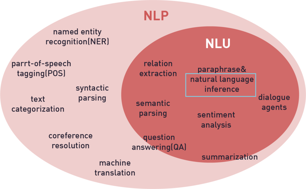
How NLI is different from NLP?
The main difference between NLP and NLI is that NLP is a broader set that contains two subsets Natural Language Understanding (NLU) and Natural Language Generation (NLG). We are more concerned about NLU as NLI comes under this. NLU is basically making the computer capable of comprehending what the given text block represents. NLI, which comes under NLU is the task of understanding the given two statements and categorizing them either as entailment, contradiction, or neutral sentences. When dealing with data most of the NLP tasks include pre-processing steps like removing stop words, special characters, etc. But in case of NLI, one has to just provide the model with two sentences. The model then processes the data itself and outputs the relationship between the two sentences.
NLI is been used in many domains like banking, retail, finance, etc. It is widely used in cases where there is a requirement to check if generated or obtained result from the end-user follows the hypothesis. One of the use cases includes automatic auditing tasks. NLI can replace human auditing to some extent by comparing if sentences in generated document entail with the reference documents.
Models used to Demonstrate NLI Task
In this blog, I have demonstrated the NLI task using two models: RoBERTa and XLM-RoBERTa. Let us understand these models in this section.
In order to understand RoBERTa model, one should have a brief knowledge about BERT model.
BERT
Bidirectional Encoder Representation Transformers (BERT) was published by Google AI researchers in 2018. It has shown state-of-the-art results in many NLP tasks like question and answering, NLI task etc. It is basically an encoder stack of transformer architecture. It has two versions BERT base and BERT large. BERT base has 12 layers in its encoder stack and 110M total parameters whereas BERT large has 24 layers and 340M total parameters.
BERT pre-training consists of two tasks:
Masked Language Model (MLM)
Next Sentence Prediction (NSP)
Masked LM
In the input sequence sent to the model as input, randomly 15% of the words are masked and the model is tasked to predict these masks by understanding the context from unmasked words at the end of training. This helps model in understanding the context of the sentence.
Next Sentence Prediction
Model is fed with two-sentence pairs as input. In this task, a model must predict at the end of training whether the sentences follow or unfollow each other. This helps in understanding the relationship between two sentences which is the major objective for tasks like question and answering, NLI, etc.
Both the tasks are executed simultaneously while training.
Model Input
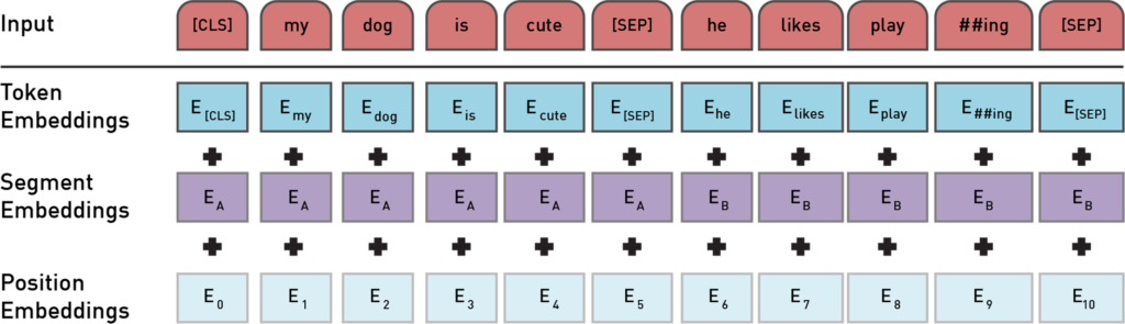
Input to the BERT model is a sequence of tokens that are converted to embeddings. Each token embedding is a combination of 3 embeddings.
Figure 2: BERT input representation [1]
Token Embeddings – These are word embeddings from WordPiece token vocabulary.
Segment Embeddings – As BERT model takes pair of sentences as input, in order to help model distinguish the embeddings from different sentences these embeddings are used. In the above picture, EA represents embeddings of sentence A while EB represents embeddings from sentence B.
Position Embeddings – In order to capture “sequence” or “order” information these embeddings are used to express the position of words in a sentence.
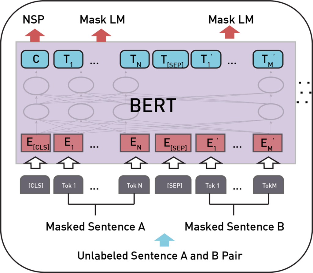
Model Output
The output of BERT model has the same no. of tokens as input with additional classification token which gives the classification results ie. whether sentence B follows sentence A or not.
Figure 3: Pre-training procedure of BERT [1]
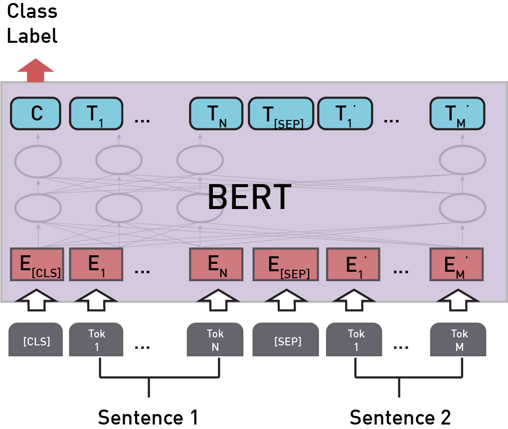
Fine-Tuning BERT
A pre-trained BERT model can be fine-tuned to achieve a specific task on specific data. Fine-tuning uses same architecture as the pre-trained model only an additional output layer is added depending on the task. In case of NLI task classification token is fed into the output classification layer which determines the probabilities of entailment, contradiction, and neutral classes.
Figure 4: Illustration for BERT fine-tuning on sentence pair specific tasks like MNLI, QQP, QNLI, RTE, SWAG etc. [1]
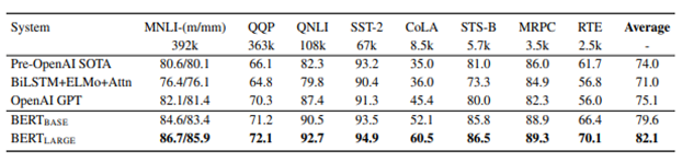
BERT GLUE Task Results
Figure 5: GLUE test results [1]
As you can see in figure 4, BERT outperforms all the previous models on GLUE tests.
RoBERTa
Robustly Optimised BERT Pre-training Approach (RoBERTa) was proposed by Facebook researchers. They found with a much more robustly pre-training BERT model it can still perform better on GLUE tasks. RoBERTa model is a BERT model with modified pre-training approach.
Below are the few changes incorporated in RoBERTa model when compared to BERT model.
Data – RoBERTa model is trained using much more data when compared to BERT. It is trained on 160GB uncompressed data.
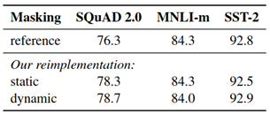
Static vs Dynamic Masking – In BERT model, data was masked only once during pre-processing which results in single static masks. These masks are used for all the iterations while training. In contrast, data used for RoBERTa training was duplicated 10 times with 10 different mask patterns and was trained over 40 epochs. This means a single mask pattern is used only in 4 epochs. This is static masking. While in dynamic masking different mask pattern is generated for every epoch during training.
Figure 6: Static vs Dynamic masking results [2]
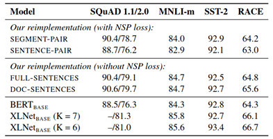
3. Removal of Next Sentence Prediction (NSP) objective – Researches have found that removing NSP loss significantly improved the model performance on GLUE tasks.
Figure 7: Model results comparison when different input formats are used [2]
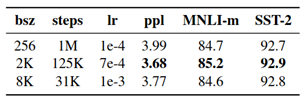
4. Trained on Large Batch Sizes – Training model on large batch sizes improved the model accuracy.
Figure 8: Model results when trained with different batch sizes [2]
5. Tokenization – RoBERTa uses a byte-level Byte-Pair Encoding (BPE) encoding scheme with a containing 50K vocabulary in contrast to BERT’s character-level BPE with a 30K vocabulary.
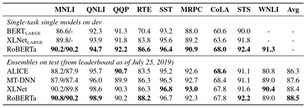
Figure 9: RoBERTa results on GLUE tasks. [2]
RoBERTa Results on GLUE Tasks
RoBERTa clearly outperforms when compared to previous models.
XLM-RoBERTa
XLM-R is a large multilingual model trained on 100 different languages. It is basically an update to Facebook XLM-100 model which is also trained in 100 different languages. It uses the same training procedure as RoBERTa model which used only Masked Language Model (MLM) technique without using Next Sentence Prediction (NSP) technique.
Noticeable changes in XLM-R model are:
Data – XLM-R model is trained on large cleaned CommonCrawl data scaled up to 2.5TB which is a way larger than Wiki-100 corpus which was used in training other multilingual models.
Vocabulary – XLM-R vocabulary contains 250k tokens in contrast to RoBERTa which has 50k tokens in its vocabulary. It uses one large shared Sentence Piece Model (SPM) to tokenize words of all languages instead of XLM-100 model which uses different tokenizers for different languages. XLM-R authors assume that similar words across all the languages have similar representation in space.
XLM-R is self-supervised, whereas XLM-100 is supervised model. XLM-R samples stream of text from each language and trains the model to predict masked tokens. XLM-100 model required parallel sentences (sentences that have same meaning) in two different languages as input which is a supervised method.
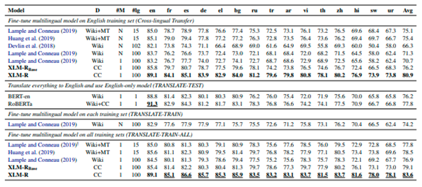
XLM-R Results on Cross-Lingual-Classification on XNLI dataset
Figure 10: XLM-R results on XNLI dataset. [3]
XLM-R is now the state-of-the-art multilingual model which outperforms all the previous multi-language models.
Demonstration of NLI Task Using Kaggle Dataset
In this section, we will implement the NLI task using Kaggle dataset.
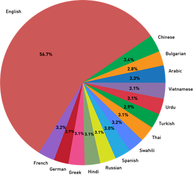
Kaggle has launched Contradictory My Dear Watson challenge to detect contradiction and entailment in multilingual text. It has shared a training and validation dataset that contains 12120 and 5195 text pairs respectively. This dataset contains textual pairs from 15 different languages – Arabic, Bulgarian, Chinese, German, Greek, English, Spanish, French, Hindi, Russian, Swahili, Thai, Turkish, Urdu, and Vietnamese. Sentence pairs are classified into three classes entailment (0), neutral (1), and contradiction (2).
We will be using the training dataset of this challenge to demonstrate the NLI task. One can run the following code blocks using Google Colab and can download a dataset from this link.
Code Flow
1. Install transformers library
!pip install transformers
2. Load XLM-RoBERTa model –
Since our dataset contains multilingual text, we will be using XLM-R model for checking the accuracy on training dataset.
from transformers import AutoModelForSequenceClassification, AutoTokenizer xlmr= AutoModelForSequenceClassification.from_pretrained(‘joeddav/xlm-roberta-large-xnli’) tokenizer = AutoTokenizer.from_pretrained(‘joeddav/xlm-roberta-large-xnli’)
3. Load training dataset –
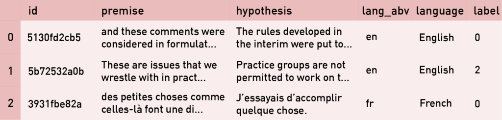
import pandas as pd train_data = pd.read_csv(<dataset path>) train_data.head(3)
4. XLM-R model classes –
Before going further do a sanity check to confirm if the model classes notation and the dataset classes notation is same
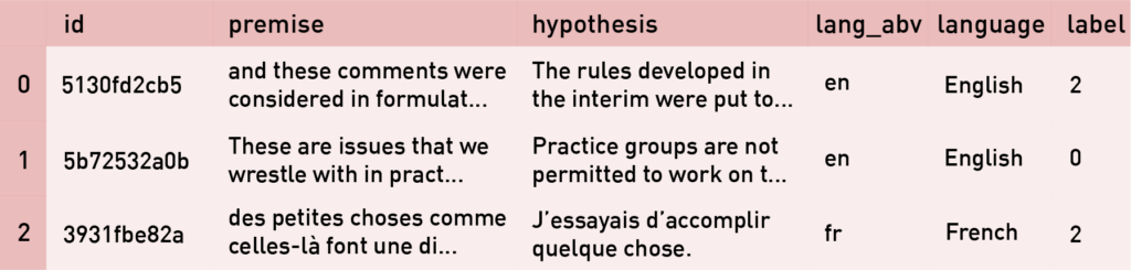
We can see that the model classes notation and Kaggle dataset classes notation (entailment (0), neutral (1), and contradiction (2)) is different. Therefore, change the training dataset classes notation to match with model.
Check the distribution of training data based on language
train_data_lang = train_data.groupby(‘language’).count().reset_index()[[‘language’,’id’]] # plot pie chart import matplotlib.pyplot as plt import numpy as np plt.figure(figsize=(10,10)) plt.pie(train_data_lang[‘id’], labels = train_data_lang[‘language’], autopct=’%1.1f%%‘) plt.title(‘Distribution of Train data based on Language’) plt.show()
We can see that English constitutes to more than 50% of the training data.
7. Sample data creation –
Since training data has 12120 textual pairs, evaluating all the pairs would be time-consuming. Therefore, we will create a sample data out of training data which will be a representative sampling ie. sample data created will have the same distribution of text pairs based on language as of the training data.
# create a column which tells how many random rows should be extracted for each language train_data_lang[‘sample_count’] = train_data_lang[‘id’]/10 # sample data sample_train_data = pd.DataFrame(columns = train_data.columns) for i in range(len(train_data_lang)): df = train_data[train_data[‘language’] == train_data_lang[‘language’][i]] n = int(train_data_lang[‘sample_count’][i]) df = df.sample(n).reset_index(drop=True) sample_train_data = sample_train_data.append(df) sample_train_data = sample_train_data.reset_index(drop=True) # plot distribution of sample data based on language sample_train_data_lang = sample_train_data.groupby(‘language’).count().reset_index()[[‘language’,’id’]] plt.figure(figsize=(10,10)) plt.pie(sample_train_data_lang[‘id’], labels = sample_train_data_lang[‘language’], autopct=’%1.1f%%‘) plt.title(‘Distribution of Sample Train data based on Language’) plt.show()
We can see that sample data created and the training data have nearly same distribution of text pairs based on language.
8. Functions to get predictions from XLM-R model –
def get_tokens_xlmr_model(data): ”’ Function which creats tokens for the passed data using xlmr model input – Dataframe Output – list of tokens ”’ batch_tokens = [] for i in range(len(data)): tokens = tokenizer.encode(data[‘premise’][i], data[‘hypothesis’][i], return_tensors=’pt’, truncation_strategy=’only_first’) batch_tokens.append(tokens) return batch_tokens def get_predicts_xlmr_model(tokens): ”’ Function which creats predictions for the passed tokens using xlmr model input – list of tokens Output – list of predictions ”’ batch_predicts = [] for i in tokens: predict = xlmr(i)[0][0] predict = int(predict.argmax()) batch_predicts.append(predict) return batch_predicts
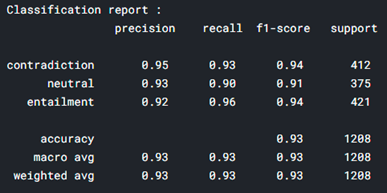
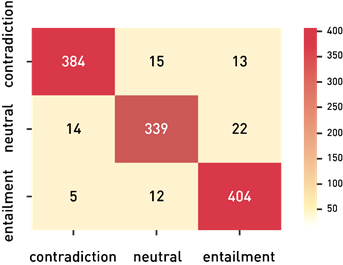
# plot the confusion matrix and classification report for original labels to the predicted labels import numpy as np import seaborn as sns from sklearn.metrics import classification_report sample_train_data[‘label’] = sample_train_data[‘label’].astype(str).astype(int) x = np.array(sample_train_data[‘label’]) y = np.array(sample_train_data_predictions) cm = np.zeros((3, 3), dtype=int) np.add.at(cm, [x, y], 1) sns.heatmap(cm,cmap=”YlGnBu”, annot=True, annot_kws={‘size’:16}, fmt=’g’, xticklabels=[‘contradiction’,’neutral’,’entailment’],
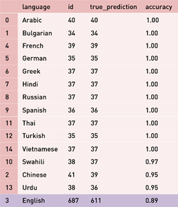
Except for English, rest of the languages are having accuracy greater than 94%. Therefore, use a different model for English pairs prediction to further improve accuracy.
12. RoBERTa model for English text pairs prediction –
14. Functions to get predictions from RoBERTa model –
def get_tokens_roberta(data): ”’ Function which generates tokens for the passed data using roberta model input – Dataframe Output – list of tokens ”’ batch_tokens = [] for i in range(len(data)): tokens = roberta.encode(data[‘premise’][i],data[‘hypothesis’][i]) batch_tokens.append(tokens) return batch_tokens def get_predictions_roberta(tokens): ”’ Function which generates predictions for the passed tokens using roberta model input – list of tokens Output – list of predictions ”’ batch_predictions = [] for i in range(len(tokens)): prediction = roberta.predict(‘mnli’, tokens[i]).argmax().item() batch_predictions.append(prediction) return batch_predictions
sample_train_data_en[‘prediction’] = sample_train_data_en_predictions # roberta model accuracy sample_train_data_en[‘true_prediction’] = np.where(sample_train_data_en[‘label’]==sample_train_data_en[‘prediction’], 1, 0) roberta_accuracy = round(sum(sample_train_data_en[‘true_prediction’])/len(sample_train_data_en), 2) print(“Accuracy of RoBERTa model {}“.format(roberta_accuracy))
Accuracy of RoBERTa model 0.92
Accuracy of English text pairs increased from 89% to 92%. Therefore, for predictions on test dataset of Kaggle challenge use RoBERTa for English pairs prediction and XLM-R for predictions of other language pairs.
By this approach, I was able to score 94.167% accuracy on the test dataset.
Conclusion
In this blog ,we have learned what NLI task is, how to achieve this using two state-of-the-art models. There are many more pre-trained models for achieving NLI tasks other than the models discussed in this blog. Few of them are language-specific like German BERT, French BERT, Finnish BERT, etc. multilingual models like Multilingual BERT, XLM-100, etc.
As future steps, one can further achieve task-specific accuracy by finetuning these models with specific data.
In-store traffic analytics allows data-driven retailers to collect meaningful insights about customer’s behavioral data.
The retail industry receives millions of visitors every year. Along with fulfilling the primary objective of a store, it is can also extract valuable insights from this constant stream of traffic.
The footfall data, or the count of people in a store, creates an alternate source of value for retailers. One can collect traffic data and analyze key metrics to understand what drives the sales of their product, customer behavior, preferences, and related information.
2. How does it help store potential?
Customer Purchase Experience
Store Traffic Analytics helps provide insights and in-depth knowledge of customer shopping and purchasing habits, their in-store journey, etc., by capturing key data points such as the footfall at different periods, the preferred product categories identifying traffic intensity across departments, among others. Retailers can leverage such analytics to strategize and target their customers such that it enhances customer experience and drive sales.
Customer Dwell Time Analysis
Dwell time is the length of time a person spends looking at the display or remains in a specific area. It grants an understanding of what in a store holds customer attention and helps in optimizing store layouts and product placements for higher sales.
Demographics Analysis
Demographic analysis separates store visitors into categories based on their age and gender, aiding in optimizing product listing. For instance, a footwear store footfall analysis shows that the prevalent customers are young men between the age group of 18-25. The information helps the store manager list products that appeal to this demographic group, ensuring better conversion rates.
Human Resource Scheduling
With the help of store traffic data, workforce productivity can also be enhanced by effective management of staff schedules according to peak shopping times to meet demands and provide a better customer experience, directly impacting operational costs.
3. Customer Footfall Data
The first step for Store Traffic Analytics is to have a mechanism to capture customer footfall data. Methods to count people entering the store (People Counting) have been evolving rapidly. Some of them are as follows –
Manual tracking
Mechanical counters
Pressure mats
Infrared beams
Thermal counters
Wi-Fi counting
Video counters.
This article will take a closer look into the components of an AI-based object detection and tracking framework for Video counters using Python, Deep Learning and OpenCV, by leveraging CCTV footage of a store.
4. People Counting (Video Counters)
Following are the key components involved in building a framework for people counting in CCTV footage:
Object Detection – Detecting objects (persons) in each frame or after a set of a fixed number of frames in the video.
Object Tracking – Assigning unique IDs to the persons detected and tracking their movement in the video stream.
Identifying the entry/exit area – Based on the angle of the CCTV footage, identifying the entry/exit area tracks the people entering and exiting a store.
Since object detection algorithms are computationally expensive, we can use a hybrid approach where objects are detected once every N frames (and not in each frame). And when not in the detecting phase, the objects are tracked as they move around the video frames. Tracking continues until the Nth frame, and then the object detector is re-run. We then repeat the entire process. The benefit of such an approach helps to apply highly accurate object detection algorithms without much computational burden.
4.1 Object Detection
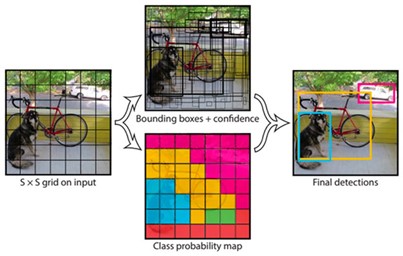
Object detection is a computer vision technique that allows us to determine where the object is in an image/frame. Some object detection algorithms include Faster R-CNN, Single Shot Detectors (SSD), You Only Look Once (YOLO), etc.
Illustration of YOLO Object Detector Pipeline (Source)
YOLO being significantly faster and accurate, can be used for video/real-time object detection. YOLOv3 model is pre-trained on the COCO dataset to classify 80 different classes, including people, cars, etc. Using the machine learning concept of transfer learning (where knowledge gained from solving a problem helps solve similar problems), for people counting, the pre-trained model weights, developed by the darknet team, can be leveraged to detect persons in the frames of the video stream.
Following are the steps involved for object detection in each frame using the YOLO model and OpenCV –
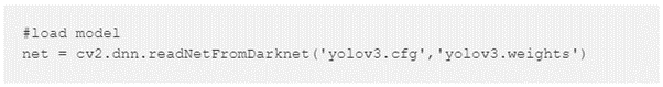
1. Load the pre-trained YOLOv3 model using OpenCV’s DNN function-
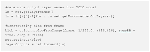
2. Determine the output layer names/classes from YOLO model and construct blob from the frame –
3. For each object detected in ‘layerOutputs,’ filter objects labeled ‘Person’ to identify all the persons present in the video frame.
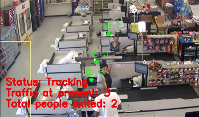
4.2 Object Tracking
The persons detected using object detection algorithms are tracked with the help of an object tracking algorithm that accepts the input coordinates (x,y) of where the person is in the frame and then assigns a unique ID to that particular person. The tracked person moves around a video stream (in different frames) by predicting the new object location in the next frame based on various factors of the frame such as gradient, speed, etc. Few object tracking algorithms are Centroid Tracking, Kalman Filter tracking, etc.
Since the position of a person in the next frame is determined to a great extent by their velocity and position in the current frame, the Kalman Filter tracking algorithm tracks old or new persons detected. Kalman Filter allows model tracking based on velocity and position, predicting likely possible positions. It does so by using Gaussians. When it receives a new reading, it uses probability to assign measurements to its prediction and update itself. Accordingly, the object assigns to existing or unique IDs. This blog explains the maths behind Kalman Filter.
4.3 Identifying the entry/exit area
To keep track of people entering/exiting a particular area of the store, based on the CCTV angle, the entry/exit area in the video stream is specified to accurately collect data of the customer journey and traffic in the store.
In the image below (the checkout counter), the yellow boundary specifies the entry/exit area, and the status of store traffic is updated accordingly.
Some key challenges observed during object detection and tracking framework for footfall data capturing are listed below –
Speed for real-time detection – The object detection and prediction time needs to be incredibly fast to accurately capture the traffic in the store with frequently visiting customers.
The angle of CCTV Cameras – The camera angle should accurately capture the footfall traffic.
Video Clarity – For object detection and tracking algorithms to accurately capture the people in a video, the quality of the video plays an important role. It should not be too blurry, have proper lighting, etc.
6. Conclusion
The need for Store Traffic Analytics has become apparent with the growing complexity of the industry. Retail businesses face fierce competition that pressures them to guarantee that the right products and services are available to their customers.
Collecting and analyzing data that accurately reveals customer behavior has therefore become a crucial part of the process.
Lorem Ipsum is simply dummy text of the printing and typesetting industry. Lorem Ipsum has been the industry's standard dummy text ever since the 1500s, when an unknown printer took a galley of type and scrambled it to make a type specimen book. It has survived not only five centuries, but also the leap into electronic typesetting, remaining essentially unchanged.