Revealing the Secrets of Creating New Game Characters Without Using Paintbrush

Introduction

In the gaming industry, the studios are responsible for the design and development of any game. A game designer will be responsible for providing multiple design ideas for various In-game components like characters, maps, scenes, weapons, etc.To develop a single character, a designer has to factor in multiple attributes like face morphology, gender, skin tone, clothing accessories, expressions, etc leading to a long and tedious development cycle. To minimize this complexity, we aim to identify tools and techniques, which can combine the automation power of machines to generate designs based on certain guard rails defined by the designers. This approach will be a path towards machine creativity with human supervision. From a business point of view, there will be more design options for the studios to select within a short span of time leading to huge cost savings.

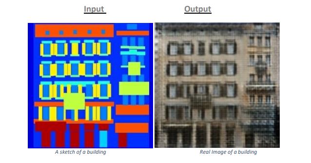
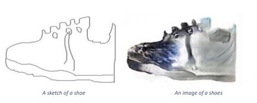
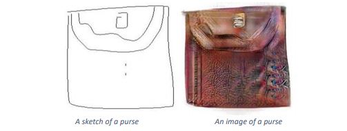
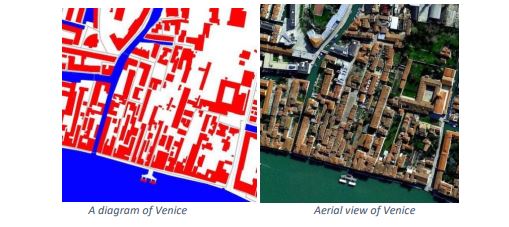
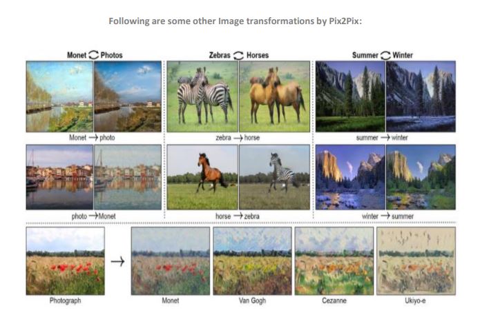
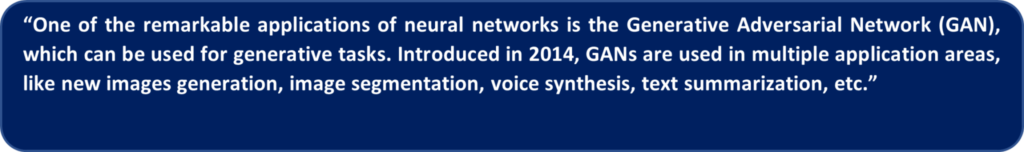
Our solution utilizes advantage of advance deep learning models like GANs which have been proven to work extremely well in generative tasks (generating new data instances) such as image generation, image-to-image translation, voice synthesis, text-to-image translation, etc.

In this whitepaper, we explore the effectiveness of GANs for a specific use case in the gaming industry. The objective of using GAN in this use case is to create new Mortal Kombat (MK) game characters through style transfer on new or synthesized images and conditional GANs to generate only the characters of interest.

GAN & it’s clever way of training a generative model for image generation!

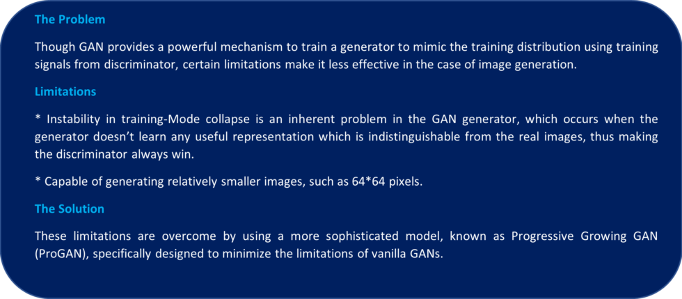
GAN has two competing neural networks, namely a Generator (G) and a Discriminator (D). In the case of image generation, the goal of the generator is to generate images that are indistinguishable (or the fake images) from the training images (or the real images). The goal of the discriminator is to classify between the fake and real images. The training process aims towards making the generator fool the discriminator, hence, to get the generated fake images that are as realistic as the real ones.

Following are the highlights of the GANs solution framework to create new Mortal Kombat Game characters without using a paintbrush:

i) Showing detailed analysis and the effectiveness of GANs to generate new MK characters in terms of image quality produced (subjective evaluation) and FID distances (objective evaluation).

ii) Results of style mixing using MK characters. The style mixing performed using the trained model.

iii) Experimental evaluation using Mortal Kombat dataset (custom dataset having 25,000) images. The training time is captured to understand the computation resources required to achieve the desired performance.

Types of GAN and their role in creating Mortal Kombat realistic characters

GANs are an advanced and rapidly changing field backed by unsupervised machine learning methodology. In order to use GAN effectively to create Mortal Kombat realistic characters, it is vital to comprehend its architecture and different types in use to get near-perfect results. In this section, we will discuss the types of GAN and architectural details of StyleGans in the latter stage.

Types of GAN

1. GAN (or vanilla GAN) [Goodfellow et al. 2014]-GAN belongs to a class of methods used for learning generative models based on game theory. There are two competing neural networks, Generator (G) and Discriminator (D). The goal of GAN is to train a generator network to produce sample distribution, which mimics the distribution of the training data. The training signal for G provided by the discriminator D, that is trained to classify the real and fake images. The following is the cost function of GAN.

Cost function:

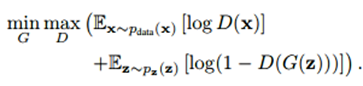
The min/max cost function aims to train the D to minimize the probability of the data generated by G (fake data) and maximize the probability of the training data (real data). Both G and D are trained in alternation by Stochastic Gradient Descent (SGD) approach.

ii) Progressive Growing GAN(ProGAN)- ProGANs (Karras et al., 2017) are capable of generating high-quality photorealistic images, starting with generating very small images of resolution 4*4, growing progressively into generating images of 8*8,…1024*1024, until the desired output size, is generated. The training procedure includes cycles of fine-tuning and fading-in, which means that there are periods of fine-tuning a model with a generator output, followed by a period of fading in new layers in both G and D.

iii) Style GANs– StyleGANs (Karras et al., 2019) are based on ProGANs with minimal changes in the architectural design to equip it to demarcate and control high-level features like pose, face shape in a human face, and low-level features like freckles, pigmentation, skin pores, and hair. The synthesis of new images controlled by the inclusion of high-level and low-level features. And it is executed by a style-based generator in styleGAN. In a style-based generator, the input to each level is modified separately. Thus, there is a better control over the features expressed at that level.

There are various changes incorporated in styleGAN generator architecture to synthesize photorealistic images. These are bilinear up-sampling, mapping network, Adaptive Instance Normalization, removal of latent point input, the addition of noise, and mixing regularization control. The intent of using StyleGan here is to separate image content and style content from the image.

(Note: For generating MK characters, we have used styleGAN architecture, and the architectural details are provided in the next section.)

iv) Conditional GANs

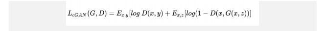
If we need to generate new Mortal Kombat characters based on the description provided by end-users. In vanilla GANs, we don’t have control over the types of data generated. The purpose of using conditional GANs [Mirza & Osindero, 2014] is to control the images generated by the generator based on the conditional information given to the generator. Providing the label information (face mask, eye mask, gender, hat, etc.) to the generator helps in restricting the generator to synthesize the kind of images the end-user wants, i.e. “content creation based on the description”.

The cost function of conditional GAN given below:

Cost function:

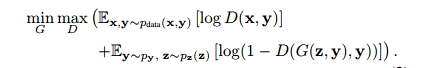
This conditional information is supplied “prior” to the generator. In other words, we are giving an arbitrary condition ‘y’ to the GAN network, which can restrict G in generating the output and the discriminator in receiving the input. The following figure depicts the cGAN inputs and an output.

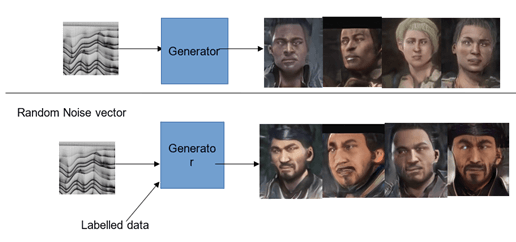
Fig 1. A- Random generation of MK characters using Random Noise vector as input, B-Controlled generation of MK characters using Random Noise vector and labeled data as input (Condition-Create MK characters with features as Male, Beard, Moustache)

Architectural details of StyleGANs

Following are the architectural changes in styleGANs generator:

  1. The discriminator D of a styleGAN is similar to the baseline progressive GAN.
  2. The generator G of a styleGAN uses baseline proGAN architecture, and the size of generated images starts from 4*4 resolution to 1024*1024 resolution on the incremental addition of layers.
  3. Bi-linear up/down-sampling is used in both discriminator and generator.
  4. Introduction of mapping network, which is used to transform the input latent vector space into an intermediate vector space (w). This process is executed to disentangle the Style and Content features. The mapping function is implemented using 8-layers Multi-layer Perceptron (8 FC in Fig 2).
  5. The output of the mapping network is passed through a learned Affine transformation (A), that transforms intermediate latent space w to styles y=(ys, yb) that controls the Adaptive Instance Normalization module of the synthesis network. This style vector gives control to the style of the generated image.
  6. The input to the AdaIN is y = (ys, yb) which is generated by applying Affine transformation to the output of the mapping network. The AdaIN operation defined as the following equation:

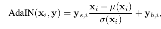
Each feature map xi is normalized separately and scaled using the scalar ys component and biased using the scalar yb component of y. The synthesis network contains 18 convolutional layers 2 for each of the resolutions for 4×4 – 1024×1024 resolution images. So, a total of 18 layers are present.

7. The input is a constant matrix of 4*4*512 dimension. Rather than taking a point from the latent space as input, there are two sources of randomness induced in generating the images. These results were extracted from the mapping network and the noise layers. The noise vector introduces stochastic variations in the generated image.
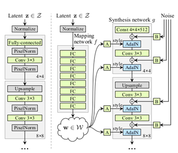
a) ProGAN generator

b) StyleGAN generator

Fig 2. a-ProGAN generator, b-StyleGAN generator [Karras et al., 2019]

Following is the table depicting different configuration setups on which style GANs can be trained.

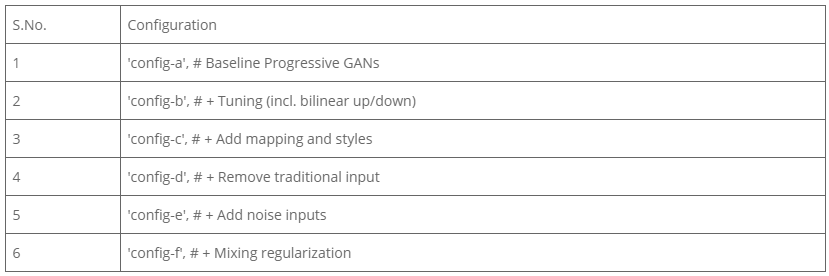
Table 1: Configuration for StyleGANs

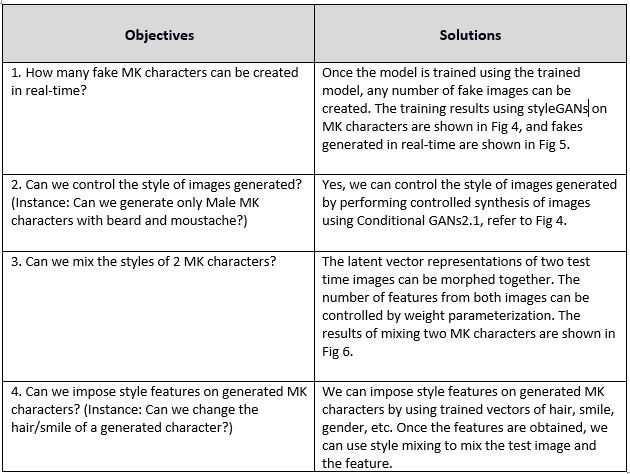
Business objectives and possible solutions

Experimental setup

Dataset

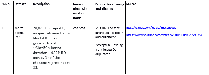
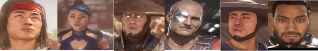
Fig 3. Sample images from the training MK dataset

Experimental design

We have conducted a set of experiments to examine the performance of StyleGANs in terms of FID, quality of output produced, training time vs performance on FID. In addition, we also checked the results imposing pre-trained latent vectors on new faces of data and Mortal Kombat characters data. We have implemented GANs and performed its feasibility analysis to overcome the following issues:

i) How effective StyleGANs are in producing MK characters with lesser data, low- resolution images, lighter architecture, and less training?

ii) How computationally extensive GANs are? Are GANs expensive to train? How to estimate the time and computational resources required to generate the desired output?

iii) How well the pre-trained vectors used for style-mixing to the original images?

Evaluation metrics

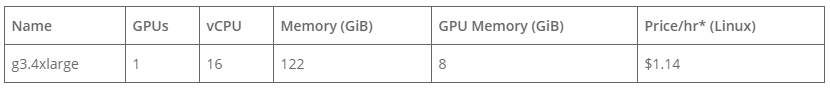
FID [Heusel et al. 2017]-Frechet Inception Distance score (FID) is a metric for image generation quality that calculates the distance between feature vectors calculated for real and generated images. FID is used to understand the quality of the image generated, the lower the FID score, higher the quality of image generated. The perfect FID score is zero. Experimental platform- All experiments are performed on the AWS platform, and the following is its configuration.

Experiments results

In order to provide a precise view of image generation of MK characters, we have conducted various experiments; and we were able to extract different results for each experiment.

  1. Training- The training images retrieved at a different number of kims are depicted in the following figures. All experiments were conducted at configuration “d”. Refer to Table 1. Fig 4. MK training results 1-Kims 2364, 2-Kims 5306 , 3-Kims 6126, 4-,Kims 8006 5-Kims 9766, 6- 10000 Kims
  1. Training time– The following table depicts the time taken, and FID results for the model trained till 10000 kims. The best-trained models have an FID of 4.88 on the FFHQ dataset (Karras et al., 2019) on configuration d (refer table 1). We got the final FID score of 53.39 on the MK dataset.

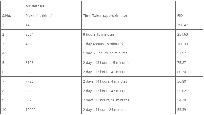
Table 3. Time taken for training & FID score

iii) Real-time image generation – Following are some of the fake images generated using different trained models using random seed values.

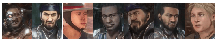
Fig 5. Real-time images generation (using seed value) @7726 kims pickle MK.

iv) Style Mixing

Using the Style Mixing method to generate new variations in the character appearance where we could use two or more reference images to generate new results. In this context, we have used two characters to create a new character.

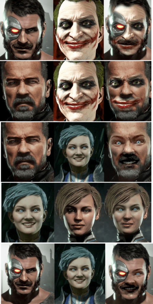
Fig 6. Style Mixing results on

MK characters

v) Progressively growing GAN- results on MK

When progressively growing GAN is applied to MK characters, with its nature of incrementally adding the layers to the network, the network learns to generate smaller and low-resolution images, followed by more complex images. Thus, stabilizing the training and overcoming mode collapse of the generators.

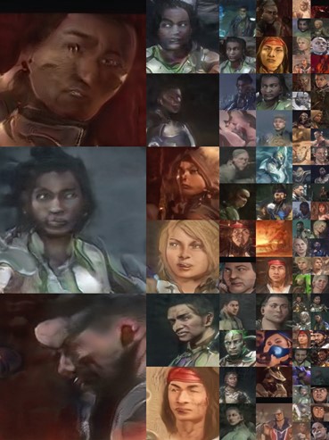
Fig 7. Progressive GANs output

Conclusion

In this whitepaper, we have discussed the methodology of applying the feasibility analysis using styleGANs for Mortal Kombat characters. We have provided a detailed report on the GANs types and evolution with respect to image generation approaches to solve different use cases using GANs. Which also includes style representation and conditional generation. The latter part of our attempt provides the results of GANs training time, FID scores, real-time image generation output, style mixing, and ProGANs results. After completing ~15 days of training (with GPU cost $1.14 per hour), the FID score achieved is 53.39. The quality of images is also improved, which can be further enhanced by conducting flawless training sessions. Recent advancements

in GANs illustrate that a better GAN performance is achievable even with fewer data. Adaptive Discriminator Augmentation [Karras et al., 2020] and Differentiable Augmentation [Zhao et al., 2020] are a few of the recent approaches which have been proposed to train GANs effectively even with less amount of data, which is currently being researched in our CoE team.

About Affine

Affine is a Data Science & AI Service Provider, offering capabilities across the analytical value chain from data engineering to analytical modeling and business intelligence to solve strategic & day-to-day business challenges of organizations worldwide. Affine is a strategic analytics partner to medium and large-sized organizations (majorly Fortune 500 & Global 1000) around the globe that creates cutting-edge creative solutions for their business challenges.

References

[1] Goodfellow, I., Pouget-Abadie, J., Mirza, M., Xu, B., Warde-Farley, D., Ozair, S., … & Bengio, Y. (2014). Generative adversarial nets. In Advances in neural information processing systems (pp. 2672-2680).

[2] Heusel, M., Ramsauer, H., Unterthiner, T., Nessler, B., & Hochreiter, S. (2017). Gans trained by a two time-scale update rule converge to a local nash equilibrium. In Advances in neural information processing systems (pp. 6626-6637).

[3] Karras, T., Aila, T., Laine, S., & Lehtinen, J. (2017). Progressive growing of gans for improved quality, stability, and variation. arXiv preprint arXiv:1710.10196.

[4] Karras, T., Laine, S., & Aila, T. (2019). A style-based generator architecture for generative adversarial networks. In Proceedings of the IEEE conference on computer vision and pattern recognition (pp. 4401-4410).

[5] Karras, T., Aittala, M., Hellsten, J., Laine, S., Lehtinen, J., & Aila, T. (2020). Training generative adversarial networks with limited data.arXiv preprint arXiv:2006.06676.

[6] Mirza, M., & Osindero, S. (2014). Conditional generative adversarial nets.arXiv preprint arXiv:1411.1784.

[7] Zhao, S., Liu, Z., Lin, J., Zhu, J. Y., & Han, S. (2020). Differentiable Augmentation for Data-Efficient GAN Training. arXiv preprint arXiv:2006.10738.

Recommendation Systems for Marketing Analytics

How I perceive recommendation systems is something which the traditional shopkeepers used to use.

Remember the time when we used to go shopping with our mother in the childhood to the specific shop. The shopkeeper used to give the best recommendations for the products, and we used to buy it from the same shop because we knew that this shopkeeper knows us best.

What the shopkeeper did was he understood our taste, priorities, the price range that we are comfortable with and then present the products which best matched our requirement. This is what the businesses are doing in the true sense now.

They want to know their customer personally by their browsing behaviour and then make them recommendation of the products that they might like, the only thing is that they want to do it on a large scale.

For example, Amazon and Netflix understand your behaviour through what you browse, add to basket and order, movies you watch and like and then recommend the best of the products which you make like with high probability.

In a nutshell, they combine what you call as the business understanding with some mathematics so that we can essentially know and learn about the products that the customer likes.

So basically, as recommendation system for marketing analytics is a subclass of information filtering system that seeks the similarities between users and items with different combinations.

Below are some of the most widely used types of recommendation systems:

  1. Collaborative Recommendation system
  2. Content-based Recommendation system
  3. Demographic based Recommendation system
  4. Utility based Recommendation system
  5. Knowledge based Recommendation system
  6. Hybrid Recommendation system

Let us go into the most useful ones which the industry is using:

  • Content Based Recommendation System

The point of content-based is that we should know the content of both user and item. Usually we construct user-profile and item-profile using the content of shared attribute space. The product attributes like image (Size, dimension, colour etc…) and text description about the product is more inclined towards “Content Based Recommendation”.

This essentially means that based upon the content that I watch on Netflix, I can run an algorithm to see what the most similar movies are and then recommend the same to the other users.

For example, when you open Amazon and search for a product, you get the similar products pop up below which is the item-item similarity that they have computed for the overall products that are there in Amazon. This gives us a very simple yet effective idea of how the products behave with each other.

Bread and butter could be similar products in the true sense as they go together but their attributes can be varied. In case of the movie industry, features like genres, reviews could tell us the

similar movies and that is the type of similarity we get for the movies.

  • Collaborative Recommendation System:

Collaborative algorithm uses “User Behaviour” for recommending items. They exploit behaviour of other users and items in terms of transaction history, ratings, selection, purchase information etc. In this case, features of the items are not known.

When you do not want to see what the features of the products are for calculating the similarity score and check the interactions of the products with the users, you call it as a collaborative approach.

We figure out from the interactions of the products with the users what are the similar products and then take a recommendation strategy to target the audience.

Two users who watched the same movie on Netflix can be called similar and when the first user watches another movie, the second users gets that same recommendation based on the likes that these people have.

  • Hybrid Recommendation System:

Combining any of the two systems in a manner that suits the industry is known as Hybrid Recommendation system. It combines the strengths of more than two Recommendation system and eliminates any weakness which exist when only one recommendation system is used.

When we only use Collaborative Filtering, we have a problem called as “cold start” problem. As we take into account the interaction of users with the products, if a user comes to the website for the first time, I do not have any recommendations to make to that customer as I do not have interactions available.

To eliminate such a problem, we used hybrid recommendation systems which combines the content-based systems and

collaborative based systems to get rid of the cold start problem. Think of it as this way, item-item and user-user, user-item interaction all combined to give the best recommendations to the users and to give more value to the business.

From here, we will focus on the Hybrid Recommendation Systems and introduce you to a very strong Python library called lightfm which makes this implementation very easy.

LightFM:

The official documentation can be found in the below link:

lyst/lightfm

Build status Linux OSX (OpenMP disabled) Windows (OpenMP disabled) LightFM is a Python implementation of a number of…

github.com

LightFM is a Python implementation of the number of popular recommendation algorithms for both implicit and explicit feedback.

User and item latent representations are expressed in terms of their feature’s representations.

It also makes it possible to incorporate both item and user metadata into the traditional matrix factorization algorithms. When multiplied together, these representations produce scores for every item for a given user; items scored highly are more likely to be interesting to the user.

Interactions : The matrix containing user-item interactions.

User_features : Each row contains that user’s weights over features.

Item_features : Each row contains that item’s weights over features.

Note : The matrix should be Sparsed (Sparse matrix is a matrix which contains very few non-zero elements.)

Predictions

fit_partial : Fit the model. Unlike fit, repeated calls to this method will cause training to resume from the current model state.

Works mainly for the new users to append to the train matrix.

Predict : Compute the recommendation score for user-item pairs.

The scores are sorted in the descending form and top n-items are recommended.

Model evaluation

AUC Score : In the binary case (clicked/not clicked), the AUC score has a nice interpretation: it expresses the probability that a randomly chosen positive item (an item the user clicked) will be ranked higher than a

randomly chosen negative item (an item the user did not click). Thus, an AUC of 1.0 means that the resulting ranking is perfect: no negative item is ranked higher than any positive item.

Precision@K : Precision@K measures the proportion of positive items among the K highest-ranked items. As such, this is focused on the ranking quality at the top of the list: it does not matter how good or bad the rest of your ranking is as long as the first K items are mostly positive.

Ex: Only one item of your top 5 item are correct, then your precision@5 is 0.2

Note : If the first K recommended items are not available anymore (say, they are out of stock), and you need to move further down the ranking. A high AUC score will then give you confidence that your ranking is of high quality throughout.

Enough of the theory now, we will move to the code and see how the implementation for lightfm works:

I have taken the dataset from Kaggle, you can download it below:

E-Commerce Data

Actual transactions from UK retailer www.kaggle.com

Hope you liked the coding part of it, and you are ready to implement that in any version. The enhancement that can be done in this is if you have the product and the user features.

These can also be taken as inputs into the lightfm model and the embedding that the model creates would be based upon all those attributes. The more data that is pushed into the lightfm will give the model a better accuracy and more training data.

That’s all from my end for now. Keep Learning!! Keep Rocking!!

CatBoost – A new game of Machine Learning

Gradient Boosted Decision Trees and Random Forest are one of the best ML models for tabular heterogeneous datasets.

CatBoost is an algorithm for gradient boosting on decision trees. Developed by Yandex researchers and engineers, it is the successor of the MatrixNet algorithm that is widely used within the company for ranking tasks, forecasting and making recommendations. It is universal and can be applied across a wide range of areas and to a variety of problems.

Catboost, the new kid on the block, has been around for a little more than a year now, and it is already threatening XGBoost, LightGBM and H2O.

Why Catboost?

Better Results

Catboost achieves the best results on the benchmark, and that’s great. Though, when you look at datasets where categorical features play a large role, this improvement becomes significant and undeniable.

GBDT Algorithms Benchmark

Faster Predictions

While training time can take up longer than other GBDT implementations, prediction time is 13–16 times faster than the other libraries according to the Yandex benchmark.

Left: CPU, Right: GPU

Batteries Included

Catboost’s default parameters are a better starting point than in other GBDT algorithms and it it is good news for beginners who want a plug and play model to start experience tree ensembles or Kaggle competitions.

GBDT Algorithms with default parameters Benchmark

Some more noteworthy advancements by Catboost are the features interactions, object importance and the snapshot support.In addition to classification and regression, Catboost supports ranking out of the box.

Battle Tested

Yandex is relying heavily on Catboost for ranking, forecasting and recommendations. This model is serving more than 70 million users each month.

The Algorithm

Classic Gradient Boosting

Gradient Boosting on Wikipedia

Catboost Secret Sauce

Catboost introduces two critical algorithmic advances – the implementation of ordered boosting, a permutation-driven alternative to the classic algorithm, and an innovative algorithm for processing categorical features.

Both techniques are using random permutations of the training examples to fight the prediction shift caused by a special kind of target leakage present in all existing implementations of gradient boosting algorithms.

Categorical Feature Handling

Ordered Target Statistic

Most of the GBDT algorithms and Kaggle competitors are already familiar with the use of Target Statistic (or target mean encoding). It’s a simple yet effective approach in which we encode each categorical feature with the estimate of the expected target y conditioned by the category. Well, it turns out that applying this encoding carelessly (average value of y over the training examples with the same category) results in a target leakage.

To fight this prediction shift CatBoost uses a more effective strategy. It relies on the ordering principle and is inspired by online learning algorithms which get training examples sequentially in time. In this setting, the values of TS for each example rely only on the observed history.

To adapt this idea to a standard offline setting, Catboost introduces an artificial “time”— a random permutation σ1 of the training examples. Then, for each example, it uses all the available “history” to compute its Target Statistic. Note that, using only one random permutation, results in preceding examples with higher variance in Target Statistic than subsequent ones. To this end, CatBoost uses different permutations for different steps of gradient boosting.

One Hot Encoding

Catboost uses a one-hot encoding for all the features with at most one_hot_max_size unique values. The default value is 2.

Catboost’s Secret Sauce

Orederd Boosting

CatBoost has two modes for choosing the tree structure, Ordered and Plain. Plain mode corresponds to a combination of the standard GBDT algorithm with an ordered Target Statistic. In Ordered mode boosting we perform a random permutation of the training examples – σ2, and maintain n different supporting models – M1, . . . , Mn such that the model Mi is trained using only the first i samples in the permutation. At each step, in order to obtain the residual for j-th sample, we use the model Mj−1. Unfortunately, this algorithm is not feasible in most practical tasks due to the need of maintaining n different models, which increase the complexity and memory requirements by n times. Catboost implements a modification of this algorithm, on the basis of the gradient boosting algorithm, using one tree structure shared by all the models to be built.

Catboost Ordered Boosting and Tree Building

In order to avoid prediction shift, Catboost uses permutations such that σ1 = σ2. This guarantees that the target-yi is not used for training Mi neither for the Target Statistic calculation nor for the gradient estimation.

Tuning Catboost

Important Parameters

cat_features — This parameter is a must in order to leverage Catboost preprocessing of categorical features, if you encode the categorical features yourself and don’t pass the columns indices as cat_features you are missing the essence of Catboost.

one_hot_max_size — As mentioned before, Catboost uses a one-hot encoding for all features with at most one_hot_max_size unique values. In our case, the categorical features have a lot of unique values, so we won’t use one hot encoding, but depending on the dataset it may be a good idea to adjust this parameter.

learning_rate & n_estimators — The smaller the learning_rate, the more n_estimators needed to utilize the model. Usually, the approach is to start with a relative high learning_rate, tune other parameters and then decrease the learning_rate while increasing n_estimators.

max_depth — Depth of the base trees, this parameter has an high impact on training time.

subsample — Sample rate of rows, can’t be used in a Bayesian boosting type setting.

colsample_bylevel, colsample_bytree, colsample_bynode— Sample rate of columns.

l2_leaf_reg — L2 regularization coefficient

random_strength — Every split gets a score and random_strength is adding some randomness to the score, it helps to reduce overfitting.

Check out the recommended spaces for tuning here

Model Exploration with Catboost

In addition to feature importance, which is quite popular for GBDT models to share, Catboost provides feature interactions and object (row) importance

Catboost’s Feature Importance

Catboost’s Feature Interactions

Catboost’s Object Importance

SHAP values can be used for other ensembles as well

Not only does it build one of the most accurate model on whatever dataset you feed it with — requiring minimal data prep — CatBoost also gives by far the best open source interpretation tools available today AND a way to productionize your model fast.

That’s why CatBoost is revolutionising the game of Machine Learning, forever. And that’s why learning to use it is a fantastic opportunity to up-skill and remain relevant as a data scientist. But more interestingly, CatBoost poses a threat to the status quo of the data scientist (like myself) who enjoys a position where it’s supposedly tedious to build a highly accurate model given a dataset. CatBoost is changing that. It’s making highly accurate modeling accessible to everyone.

Image taken from CatBoost official documentation: https://catboost.ai/

Building highly accurate models at blazing speeds

Installation

Installing CatBoost on the other end is a piece of cake. Just run

pip install catboost

Data prep needed

Unlike most Machine Learning models available today, CatBoost requires minimal data preparation. It handles:

  • Missing values for Numeric variables
  • Non encoded Categorical variables. Note missing values have to be filled beforehand for Categorical variables. Common approaches replace NAs with a new category ‘missing’ or with the most frequent category.
  • For GPU users only, it does handle Text variables as well. Unfortunately I couldn’t test this feature as I am working on a laptop with no GPU available. [EDIT: a new upcoming version will handle Text variables on CPU. See comments for more info from the head of CatBoost team.]

Building models

As with XGBoost, you have the familiar sklearn syntax with some additional features specific to CatBoost.

from catboost import CatBoostClassifier # Or CatBoostRegressor model_cb = CatBoostClassifier() model_cb.fit(X_train, y_train)

Or if you want a cool sleek visual about how the model learns and whether it starts overfitting, use plot=True and insert your test set in the eval_set parameter:

from catboost import CatBoostClassifier # Or CatBoostRegressor model_cb = CatBoostClassifier() model_cb.fit(X_train, y_train, plot=True, eval_set=(X_test, y_test))

Note that you can display multiple metrics at the same time, even more human-friendly metrics like Accuracy or Precision. Supported metrics are listed here. See example below:

Monitoring both Logloss and AUC at training time on both training and test sets

You can even use cross-validation and observe the average & standard deviation of accuracies of your model on the different splits:

Finetuning

CatBoost is quite similar to XGBoost . To fine-tune the model appropriately, first set the early_stopping_rounds to a finite number (like 10 or 50) and start tweaking the model’s parameters.

Python Newbie – Doctest

Any Software Development process consists of five stages:

  1. Requirement Analysis
  2. Design
  3. Development
  4. Testing
  5. Maintenance

Though each and every process mentioned above is important in SDLC lifecycle, this post will mainly focus on the importance of testing and enlighten on how we can use doctest a module in python to perform testing.

Importance of testing

We all make mistakes and if left unchecked, some of these mistakes can lead to failures or bugs that can be very expensive to recover from. Testing our code helps to catch these mistakes or avoid getting them into production in the first place.

Testing therefore is very important in software development.

Used effectively, tests help to identify bugs, ensure the quality of the product, and to verify that the software does what it is meant to do.

Python module- doctest

Doctest helps you test your code by running examples embedded in the documentation and verifying that they produce the expected results. It works by parsing the help text to find examples, running them, then comparing the output text against the expected value.

To make things easier, let us start by understanding the above implementation using a simple example

Python inline function

So, in the above snippet, I have written a basic inline function that adds up a number to itself.

For this function, I run manually a couple of test cases to do some basic verification (to do sanity check of my function).

Now, consider a scenario in which python can read the above output and perform the sanity check for us at the run time. This is exactly the idea behind a doctest.

Now, let’s see how we can implement one.

Let’s take a very simple example to calculate what day of the week it will be ahead of the current weekday. We write a docstring for our function which helps us to understand what our function does and what inputs it takes and so on. In this docstring, I have added couple of test cases which will be read by the doctest module at the run time while testing is carried out.

Implementation of doctest

When we run the above script from the command, we will get the foollowing output:

Doctest Output

We can see from the above snippet that all test cases mentioned in the docstring were successful as the resulted outcome matched with the expected outcome.

But what happens if any test fails, or the script does not behave as expected?

To test this, we add a false test case as we know our script can only take integers as input.

What will happen if we give a string as an input? Let us check out.

Test case with strings as input

I have used the same script but made a small change in the test case where I have passed strings as an input.

So, what is the outcome for the above test case?

Failed test case output

Voila! We can see that the doctest has clearly identified the failed test case and listed the reason for the failure of the above-mentioned test case.

Conclusion

That is all you require to get started with doctest. In this post, we have come across the power of doctest and how it makes a lot easier to carry out automated testing for most of the script. Though, many developers find doctest easier as compared to unittest because in its simplest form, there is no API to learn before using it. However, as the examples become more complex, the lack of fixture management can make writing doctest tests more cumbersome than when using unittest. But still due to the ease of its module, doctest is worth adding to our codes.

In upcoming blogs, we are going to discuss more about handy python module that can ease our task and we will also dive into some other concepts like Machine Learning and Deep Learning. Until then, keep learning!

Recommendation Systems for Beginners

Why do we need a recommendation system ?

Let us take the simplest and the most relatable example of E-commerce giant, Amazon. When we shop at Amazon, it gives us the options of bundles and products that are usually bought along with the product you are currently going to buy. For example, if you are to buy a smartphone, it recommends you to buy a back cover for the product as well.

For a second let us think and try to figure out what Amazon is trying to do in the figure below:

What does a recommendation system do ?

A recommendation system recommends you products or items that can be of your interest or liking. Let’s take another example:

It’s quite easy to notice that they are trying to sell the equipment that is generally required for a camera (memory card and the case). Now, the main question is, how do they do it for millions of items listed on their website. This is where a recommendation system comes handy.

When we first set up our Netflix account, they ask us what our preferences are, which movie or TV show is most likely to be watched by us or what genre of movie is our favorite. So as the first layer of recommendation, Netflix gives us recommendations based on our input, it shows us movies or shows similar to the input that we had provided to it. Once we are a frequent user, it has gathered enough data and gives recommendations more accurately based on our preferences of genres, cast, star rating, and so on…

The ultimate aim here is to recommend a user with an item such that he will watch it or buy it(in the case of Amazon), this in turn makes sure that the user is engaged with the platform and the customer lifetime value(CLTV) is maintained.

Objective of this blog

By the end of this blog, one will have a basic understanding of how to approach towards building a recommendation system. To make things more lucid let us take an example and try building a Hotel recommendation system. In this process, we will cover data understanding and the algorithms that can be used to realize how a nascent recommendation engine is built. We will use analogies between diurnal used products like Amazon and Netflix to have a clearer understanding.

Understanding the data required for building a recommendation system

To build a recommendation system, we must be clear with the problem statement and the end objective to provide accurate recommendations. For example, consider the following scenarios:

  1. Providing a user with a hotel recommendation based on his/her current search and historical behavior (giving a recommendation knowing that a user is looking for a hotel in Las Vegas and prefers hotels with casinos).
  2. Providing a hotel recommendation based on the user’s historical behavior, targeting those users who are not actively engaged (searching) but can be incentivized towards making a booking by targeting through a relevant recommendation (a general recommendation can be based on metrics such as a user’s historical star rating preference or historical budget preference).

These are two different objectives, and hence, the approach towards achieving both of them is different.

One must be aware of what type of data is available and also needs to know how to leverage that data to proceed towards building a recommendation engine.

There are two types of data which are of importance in our use case:

Explicit Data:

Explicit signals or input is where a user directly gives feedback to a particular item/product. This can be star values, say in the range of 1 to 5 or just a binary 1(like) and 0(dislike). For example, when we rate an item on Amazon or when we rate a movie on IMDb, these are explicit signals where we are directly giving our feedback towards an item. One thing to keep in mind is that we should be aware that each and every individual is not the same, i.e. for an Item X, User A, and User B can have different ratings. User A can be generous with his ratings and can give a rating of 5 stars whereas, User B is a critic and gives Item X 3.5 stars and gives 5 stars only for exceptional Items.

Replicating the example for our Hotel recommendation use case can be summarized like, the filters that a user applies while searching for a Hotel, say, filters like swimming pool or WiFi are explicit signals, here the user is explicitly saying that he is interested in properties which have WiFi and a swimming pool.

Additionally, the explicit data is sparse in most of the cases, as it is not ideally possible for a user to give ratings to each and every item. Logically thinking, I would not have seen each and every movie on Netflix and hence can only provide feedback for the set of movies that I have seen. These ratings reflect how much a user likes or approves of an item.

Implicit Data:

Implicit signals are obtained by capturing a user’s interaction with the item. This can be a continuous value, like the number of times a user has clicked on an item or the number of times a user has watched an Action movie or Binary, similar to just clicked or not clicked. For example, while scrolling through amazon.com the amount of time spent viewing an item or the number of times you have clicked the item can act as implicit feedback.

Drawing parallels for hotel recommendations with implicit signals can be understood as follows. Consider that we have the historical hotel bookings of a user A, and we see that in the 4 out of 5 bookings made by the user, it was a property that was near the beach. This can act as an implicit signal where we can say that user A prefers hotels near the beach.

Types of Recommendation Systems

Let us take a specific example given below to further explain the recommendation models:

While making a hotel recommendation system, we have the user’s explicit and implicit signals. However, we do not have all the signals for all the users, for a set of users E, we have explicit signals and for a set of users I, we have implicit signals.

Further, let us assume that a hotel property has the following attributes:

WiFi Availability, Couple Friendly, Budget Friendly and Nature Friendly (closer to nature)

For simplicity, let us assume that these are flags, such that if a property A has WiFi in it, the WiFi availability column will be 1. Hence our hotels data will look something like the following:

Let us name this table as Hotel_Type for further use

Content Based Filtering:

This technique is used when explicit signals are provided by the user or when we have the user and item attributes and the interaction of the user with that item. The objective here is to show items/products which are similar to the item/product that a person has already purchased or shows a liking for, or in another case, show a product to a user where he explicitly says that he is looking for something in particular. Taking our example, consider that you are booking a hotel from xyz.com, you apply filters for couple-friendly properties, here you are explicitly saying that you are looking for a couple-friendly property and hence, xyz.com will show you properties that are couple friendly. Similarly, while providing recommendations, if we have explicit signals from a user we try to get the best match for that signal with the list of items that we have and provide recommendations accordingly.

Model Algorithms:

Cosine Similarity: It is a measure of similarity

between two non-zero vectors. The values range from 0 to 1.

Cosine Similarity is used as a measure of similarity between two non-zero vectors. Here the vectors can be both user or item based.

Let us take an example, Assume that a user A has specifically shown interest towards property X from the hotel_type table (the user has previously booked the property or has searched for the property X multiple times recently), we now have to recommend him properties that are similar to property X. To do so, we are going to find the similarity between property X and the rest of the properties in the table.

We can clearly see that property Q has the highest similarity with property X and followed by property P. So if we are to recommend a property to user A, we will recommend him property Q knowing that he has a preference for property X.

Pearson Correlation: It is a measure of linear correlation between two variables. The values range from -1 to 1.

Let us take an example where we are getting explicit input from the user where the user is shown the 4 categories (WiFi, Budget, Couple, Nature). The user has the option to provide his input by selecting as many as he wants, he can even select none. Considering the case when a user B has selected at least one of the 4 options. Now, assume user B’s input looks like the following:

While one can say that we can use cosine similarity in this case by just filling in the null values as 0. However, it is not advised to do so since, cosine similarity assumes the 0’s as a negative preference and in this explicit signal we cannot for sure say that user B is not looking for a couple friendly or a budget friendly property just because the user has not given an input in that field.

Hence, to avoid this, we use Pearson correlation and the output of the similarity measuring technique would look like the following:

We can see that property Z is highly correlated to user B’s explicit signal and hence, we will provide Z as a recommendation for user B.

So, for the set of users E (explicitly proving us their preference) we will use Pearson Correlation and for the set of users I (implicitly telling us that he/she is looking for a property with a certain set of attributes), we will use Cosine Similarity.

Note: A user’s explicit signal is always preferred over an implicit signal. For example, in the past, I have only booked hotels in the urban areas, however, now I want to book a hotel near the beach (nature friendly). In my explicit search, I specify this, but if you are making an implicit signal from my past bookings you will see that I do not prefer hotels near the beach and would recommend me hotels in the city. In conclusion, Pearson correlation and Cosine similarity are the most widely used similarity techniques, however, we need to always use the correct similarity measuring technique as per our use case. More information on different types of similarity techniques can be found here.

Collaborative Filtering:

This modeling technique is used by leveraging user-item interaction. Here, we try to match or group similar users and recommend based on the preferences of similar users. Let us consider a user-item interaction matrix (rating matrix) where we have the hotel rating a user has given a particular hotel:

Rating Matrix

Now let us compare user A and user E, we can see that they both have similar tastes and have rated Hotel Y as 4, seeing this let us assume that user A will rate Hotel X as 5 and hotel R as 3. Hence, we can give a recommendation of hotel X to user A by noticing the similarity between user A and user E (considering that he will like Hotel X and rate it 5).

So, if we are provided with the interaction of a user with an item where the user has given feedback towards the item, we can use collaborative filtering (for example, the rating matrix). Explicit ratings such as star rating

given by the user or Implicit signals such as a flag if the user has booked a property or contrary of user-item interaction.

Model Algorithms:

Memory and Model-Based Approach are the two types of techniques to implement collaborative filtering. The key difference between the two is that in the memory-based approach we do not use parametric machine learning models.

Memory-Based Approach: It can be divided into two subdivisions, user-item filtering, and item-item filtering. In the user-item approach, we identify clusters of similar users and utilize the interaction of a particular user in that cluster to predict the interaction of the whole cluster. For example, to predict the rating user C gives to a hotel X, we will take a weighted sum of hotel X’s rating by the other users, here weight is the similarity number between user X and the other users. Adjusted cosine similarity can also be used to remove the difference in the nature of individuals, which brings critics and the general public on the same scale.

Item-item filtering is similar to user-item filtering, but here we take an item and see the users that liked that item and find other sets of items that those set of users or similar users also liked. It takes items, finds similar items, and outputs those items as recommendations.

Model-Based Approach: In this technique, we use machine learning models to predict the rating for an item that could have been given by a user and hence, provide recommendations.

Several ML models that are used, to name a few, Matrix factorization, SVD (singular value decomposition), ALS, and SVD++. Some also use neural networks, decision trees, and latent factor models to enhance the results. We will delve into Matrix Factorization below.

Matrix Factorization:

In matrix factorization, the goal is to complete the matrix and fill in the null values in the rating matrix.

The preferences of the users are identified by a small number of hidden features of the user and items. Here there are two hidden feature vectors for users(user matrix 4×2) and items(item matrix 2×4). Once we multiply the user and item matrix back together, we get back our ratings matrix with null values replaced by predicted values. Once we get the predicted values, we can recommend an Item with the highest rating for a user (not considering the items already interacted with).

Note: Here we are not providing any feature vector for the users or the items, the computation decomposes and creates vectors on its own and, finally, predicts by filling in the null values.

If we have user demographics information and user’s features and preference information and item features, we can use SVD++ where we can pass users and item feature vectors as well to get the best recommendation results.

Hybrid Models:

The hybrid model combines multiple models/algorithms to build a recommendation system. To improve the effectiveness of the recommendation, we can combine collaborative filtering and content-based filtering giving appropriate weights to the individual models and finally using this hybrid system to give out a recommendation.

For example, we can combine the results of the following by giving weights:

  1. Using Matrix factorization (collaborative filtering) on ratings matrix to match similar users and predict a rating for the user-item pair.
  2. Using Pearson correlation (content-based filtering) to find similarity between users who provide explicit filters and the hotels with feature vectors.

The combined results can be used to provide recommendations to users.

Conclusion:

Building a recommendation system highly depends on the end objective and the data we have at hand. Understanding the algorithms and knowing which one to use to get recommendations plays a vital role in building a suitable recommendation system. Additionally, a sound recommendation system also uses multiple algorithms and combines the results to provide the final recommendations.

References:

Bring your Art to Life with Pix2Pix

As an artist, I always wondered if I could bring my art to life. Although, it makes no sense, what if I told you that this was possible with Machine Learning? Imagine a machine learning algorithm that can convert all your sketches with a simple line of your drawing as a reference point to convert this into an oil painting based on its understanding of real-world shapes and patterns from human drawings, and photos. As an accomplished artist, your results can be quite interesting.

Pix2Pix is a Generative Adversarial Network, or GAN model designed for general purpose image-toimage translation. Image to Image translation is a problem where you have to translate a given image
domain to a target domain. For example, let’s say the input domain images are of cats, and the target
domain images are of dogs. In this case, the Image-to-Image translation algorithm learns mapping from
inputs to the target domain in such a way that if you input the image of a dog, it can change it to an
image of a cat.

Pix2pix can also be used to:

  • Convert satellite imagery into a Google Maps-style street view
  • Translate images from daytime to nighttime
  • Sketch products to product photographs. For e.g., for shoe commercials
  • Convert high intensity images into low intensity and vice-versa

Pix2Pix algorithm is one of the first successful general Image-to-Image translation algorithms that use
“Gan Loss” to generate realistic image outputs. It is shorthand for an implementation of a generic imageto-image translation using conditional adversarial networks.
Compared to other GAN models for conditional image generation, pix2pix is relatively simple and
capable of generating large, high-quality images across a variety of image translation tasks.

The comparison below should give you an idea of its potential:

The GAN architecture is comprised of a Generator Model for outputs of new plausible synthetic images,
and a Discriminator Model that classifies images as Real (from the dataset) or Fake (generated). The
discriminator model is updated directly, whereas the generator model is updated via the discriminator
model, and the two models are trained simultaneously in an adversarial process where the generator
seeks to better fool the discriminator where the discriminator seeks to better identify the counterfeit
images.

The Pix2Pix model is a type of conditional GAN, or cGAN, where the generation of the output image is
conditional based on the input, and in this case, it is a source image. The discriminator is provided with a
source image, and the target image; the model must determine whether the target is a plausible
transformation of the source image.

The Generator’s Network

Generator network uses a U-Net-based architecture. U-Net’s architecture is similar to an AutoEncoder network as it uses Encoder and the Decoder for processing .

  • U-Net’s network has skip connections between Encoder layers and Decoder layers.

As shown in the picture, the output of the first layer of Encoder is directly passed to the last layer
of the Decoder, and output of the second layer of Encoder is pass to the second last layer of
the Decoder and so on.

if there are total N layers in U-Net’s (including middle layer), then there will be a skip connection
from the kth layer in the Encoder network to the (N-k+1)th layer in the Decoder network. where 1
≤ k ≤ N/2.

‘x’ and ‘y’ represent input and output channels, respectively.

The Generator’s Architecture

The Generator network is made up of these two networks:
• The Encoder network is a downsampler
• The Decoder network is an upsampler The Generator’s Encoder Architecture
• The Encoder network of the Generator network has seven convolutional blocks
• Each convolutional block has a convolutional layer, followed by a Leaky ReLU activation function
• Each convolutional block also has a batch normalization layer except for the first layer
The Generator’s Decoder Architecture
• The Decoder network of the Generator network has seven upsampling convolutional blocks
• Each upsampling block has an upsampling layer, followed by a convolutional layer, a batch of normalization layer and a ReLU activation function There are six skip-connections in a Generator network. The concatenation happens along the channel axis.
• The output from the 1st Encoder block is concatenated to the 6th Decoder block.
• The output from the 2nd Encoder block is concatenated to the 5th Decoder block.
• The output from the 3rd Encoder block is concatenated to the 4th Decoder block.
• The output from the 4th Encoder block is concatenated to the 3rd Decoder block.
• The output from the 5th Encoder block is concatenated to the 2nd Decoder block.
• The output from the 6th Encoder block is concatenated to the 1st Decoder block.

Discriminator’s Architecture

Discriminator network uses of PatchGAN architecture. The PatchGAN network contains five convolutional blocks.

Pix2Pix Network’s Training

Pix2Pix is a conditional GANs. The loss function for the conditional GANs can be written as below:

Following are the steps that involve training the model for the Pix2Pix algorithm:

  1. Import TensorFlow and required Libraries

2. Load the Dataset

3. Input Pipeline

4. Build the Generator

• The architecture of generator is a modified U-Net.
• Each block in the encoder is (Conv -> Batchnorm -> Leaky ReLU)
• Each block in the decoder is (Transposed Conv -> Batchnorm -> Dropout (applied to the first
three blocks) -> ReLU)
• There are skip connections between the encoder and decoder (as in U-Net).

5. Generator loss

• It is a sigmoid cross entropy loss of the generated images and an array of ones
• It includes L1 loss which is MAE (mean absolute error) between the generated image and the
target image
• This allows the generated image to become structurally similar to the target image
• The formula to calculate the total generator loss = gan_loss + LAMBDA * l1_loss, where LAMBDA
= 100 l

The training procedure for the generator is shown below:

6. Build the Discriminator

  • The Discriminator is a PatchGAN.
  • Each block in the discriminator is (Conv -> BatchNorm -> Leaky ReLU)
  • The shape of the output after the last layer is (batch_size, 30, 30, 1)
  • Each 30×30 patch of the output classifies a 70×70 portion of the input image (such an architecture is called a PatchGAN).
  • Discriminator receives 2 inputs:
  • Input image and the target image, which it should classify as real.
  • Input image and the generated image (output of the generator), which it should classify as fake.
  • We concatenate these 2 inputs together in the code (tf.concat([inp, tar], axis=-1))

7. Discriminator loss

  • The discriminator loss function takes 2 inputs: real images and generated images
  • real_loss is a sigmoid cross entropy loss of the real images and an array of ones (since these are the real images)
  • generated_loss is a sigmoid cross entropy loss of the generated images and an array of zeros (since these are the fake images)
  • Then the total_loss is the sum of real_loss and the generated_loss

8.Define the Optimizers and Checkpoint-saver

9. Generate Images

Write a function to plot some images during training.

  • We pass images from the test dataset to the generator
  • The generator will then translate the input image into the output
  • Last step is to plot the prediction
  1. Training
  • For each example input, generate an output
  • The discriminator receives the input_image and the generated image as the first input. The second input is the input_image and the target_image
  • Next, we calculate the generator and the discriminator loss
  • Then, we calculate the gradients of loss with respect to both the generator and the discriminator variables (inputs) and apply those to the optimizer
  • Then log the losses to TensorBoard

The Training Loop:

  • Iterates over the number of epochs
  • On each epoch, it clears the display, and runs generate_images to show its progress
  • On each epoch it iterates over the training dataset, printing a ‘.’ for each example
  • It saves a checkpoint every 20 epochs

The beauty about a trained pix2pix network is that it will generate an output from any arbitrary input.
Following are the inputs and their corresponding outputs generated after applying Pix2Pix

Conclusion

Pix2Pix is a whole new strategy for Image-to-Image translation using a combination of the Generator and
Discriminator. It gives us chance to turn our art into life. It also proves to be useful in various spheres like
exploring satellite images and in various Augment Reality techniques. This technique could open a new
opportunity for Virtual Reality and give it a whole new approach.

Reference

  • https://arxiv.org/pdf/1611.07004.pdf
  • https://openaccess.thecvf.com/content_CVPR_2019/papers/Qu_Enhanced_Pix2pix_Dehazing_Network_CVPR_2019_paper.pdf
  • https://openaccess.thecvf.com/content_cvpr_2017/papers/Isola_Image-ToImage_Translation_With_CVPR_2017_paper.pdf

Evolution Of Human Resource In The New World Of Technology How has the Human Resources changed with time?

Of all the departments and functions in a corporate organization, Human Resource is the one function related to employees’ personal aspects. The entire employee job cycle is taken care of by the Human Resources (HR), ranging from hiring, compensation, leave management, employee satisfaction, development, and growth till exit. This function requires personal involvement and conscience that may vary from person to person.

Another rather unique aspect of an organization – technology is the practical and scientific application of various aspects such as skills, processes, methods, and organization techniques. It does not concern any personalized features and derives the same result irrespective of who, where, or when someone brings it into the organizational process.

But what if these two aspects are related?

The challenges related to HR, like Employee Engagement, Employee Retention, development of the leaders, competitive compensation, global outreach of businesses, and various other factors have stimulated extensive innovation in the HR field. For instance, more than 92% of the recruiters have turned their trust into Social Media hiring in the recent decade rather than organic hiring methods. More than 3% recruiters use “Snapchat” as a recruiting channel, moving beyond LinkedIn, Facebook, and Twitter. Below are some of such instances that bring HR and Technology together.

HR and Virtual Reality

COVID-19 has undoubtedly helped change the mindset of protagonists across the Corporate industry, especially in India. Holding appraisal meetings, taking interviews, onboarding, and even celebrations as part of work today takes place over video calls. Technology and Virtual Reality help HR with talent management, training, onboarding, and inductions, hiring, etc. as the new normal.

HR and Machine Learning Machine Learning (ML) uses algorithms for automated data analysis to create automated analytical models. HR deals with massive data sets from Recruitment and the Employee Database. ML technology helps HR improve the efficiency of initial research with dedicated hours to acquiring next-level results. So far, in Human Resources, machine learning

applications are confined mainly to the Recruitment process. However, it will be exciting to oversee the advancements in this field.

HR and Could Computing Cloud Computing ensures using a network of remote servers hosted on the internet instead of a personal computer or a local server. It helps data processing by storing and managing valuable information over the cloud, enabling the HR department to push its expertise into the middle and higher-level leadership, resulting in efficient business performance and execution. When the data on performance, attendance, track of time, etc. gets automated, the focus can be shifted to increasing productivity, transforming the HR department from being a cost center to generating revenues.

The mentioned instances are only some broad spectrum of Technology inter-dependencies in the HR department. The ever-changing and fast-paced technological advances are only making HR strive towards innovation that ultimately makes it even more indulged with technology.

Significantly, the global pandemic has altered stigmas helping people become adaptive. Several theories believe that remote working can continue as the “new normal” once we overcome this pandemic.

It can make the who’s who of the Corporate world, refine the entire workplace experience with HR as the bridge that connects extremes in an organization, exposing and expanding them with the latest technological developments.

It will be interesting to see how the Corporates fit into this new reality.

Making our Data Scientists and ML engineers more efficient (Part 2)

In the last post, we briefly touched upon the concept of MLOps and one of its elements, namely the Feature Store. We intend to cover a few more interconnected topics that are key to successful ML implementations and realizing sustained business impact.

At Affine, we ensure that a lion’s share of our focus in a ML project is on:

  1. Investing more time on building Great Features and Feature Stores (than ML algos – yes, please don’t frown upon this ? ).
  2. Setting up Robust and Reproducible Data and ML Pipelines to ensure faster and accurate Re-training and Serving.
  3. Following ML and Production Standard Coding Practices.
  4. Incorporating Model Monitoring Modules to ensure that the model stays healthy.
  5. Reserving the last hour of each business day on Documentation.
  6. And last but not the least, Regularly reciting the Magic words – Automate, Automate, Automate! ?

The following architecture is an attempt to simplify and encapsulate the above points:

This is the Utopian version of the ML architecture that every team aspires for. This approach attempts to address 3 aspects with respect to ML Training and Serving – Reproducibility, Continuous (or Inter-Connected-ness) and Collaboration.

Reproducibility of model artifacts/predictions – The ML components (Feature Engineering, Dataset Creation, ML tuning, Feature Contribution, etc.) should be build in such a way that it is simple to reproduce the output of each of those components seamlessly and accurately, at a later point in time. Now, from an application standpoint, this may be required for a root-case analysis (or model compliance) or re-trigger creation of ML pipeline on new dataset at a later point in time. However, equally importantly, if you can reproduce results accurately, it also guarantees that the ML pipeline (Data to ML training) is stable and robust! This also ultimately leads to reliable Model Serving.

Continuous Training aspect – This is known as Continuous Integration in the context of software engineering, and refers to automation of components like code merge, unit/regression testing, build, etc. to enable continuous delivery. A typical ML pipeline also comprises of several components (Feature Selection, Model Tuning, Feature Contribution, Model Validation, Model Serialization and finally Model Registry and Deployment). The Continuous aspect ensures that each module of our ML pipeline is fully automated and fully integrated (parameterized) with other modules, such that Data runs, Model Runs, and ML Deployment Runs happen seamlessly when the pipeline is re-triggered.

However, it all starts with “Collaboration” – Right Team and Right Mindset!

Before we delve deeper into each of these points, it is essential to touch upon one more topic – the need for a tightly-knit cross-functional team. It’s not pragmatic to expect the Data Scientists to handle all of the above aspects and the same is true for ML engineers. However, for a successful MLOps strategy, it’s important to get outside of our comfort zones, learn cross functional skills and collaborate closely. This means that the Data Scientists should learn to write production grade codes (modularization, testing, versioning, documentation, etc.) Similarly, the ML engineers should understand ML aspects like Feature Engineering and Model Selection to appreciate why these seemingly complex ML artifacts are critical in solving the business problem.

As for managing such a cross functional team of people that bring different niches, we need people who thrive in this knowledge-based ecosystem, where the stack keeps getting bigger every day. We need a ‘Jack of all Trades’, someone who knows a little bit of everything and possess the articulation skills to bring out the best from the team.

Getting the right cross functional team in place is the first (and unarguably the most important) piece of the puzzle. In the next article, we will go a bit deeper on each of the components described above. Please stay tuned…

Making our Data Scientists and ML Engineers more Efficient (Part 1)

There is a lot of backend grunt work involved in deploying an ML model successfully before we even begin to realize its business benefits. More than 60-70% of the effort that goes into an ML project involves what we call as the “glue work” – from EDAs to getting the QAed features/analytical dataset ready; to moving the final model to production (btw real-time deployments are a nightmare! ?). This glue work is usually the non-jazzy side of ML, but it’s what makes the models do what they are supposed to do –

  • Ensure Reproducible and Consistent Training and Serving Pipelines and Datasets
  • Ensure Upstream and Downstream QA for stable Feature Values and Predictions
  • Ensure 99.99% Availability
  • Sometimes, just re-write the entire ML serving part on a completely different server-side environment

Imagine doing the above time, and again every time a model needs to be refreshed or a new model/use case needs to be trained. The times we are living in are fluid, and so are the shelf lives of our models. The traditional approaches to building and deploying models prove to be a huge bottleneck while building models at scale, simply because there is a substantial amount of glue work.

At Affine, we are inculcating a mindset change (read MLOps) amongst our frontline DS and ML engineers to ensure faster training and deployment of ML models (Continuous Training Continuous Delivery/Deployment) across a variety of use cases.

The key to a successful MLOps implementation begins with a mindset change and motivation to adopt new practices, which may initially look like an overhead for a specific project, but guarantees tremendous gains in efficiency and business value over the mid to long run.

One such practice is the adoption of Enterprise Feature Store. For those familiar with DS/ML terminologies, this essentially is a most comprehensive Analytical Dataset that you can think of – comprises all possible features at the lowest possible granularity (think user-product-day level), and refreshed at a very frequency. Think of it as a living data source that has an ability to serve multiple ML use cases – through a simple API/SDK.

The Feature Store not only facilitates faster creation of Training AD but also Serving/Scoring AD and across multiple use cases within an org function (Ex: Marketing or Supply Chain)

What this means for Data Scientists

  • Faster Dev Cycle
  • Zero Data Errors: Feature Store being the Single Source of Truth
  • Leverage collective intellectual thought leadership from multiple DS who designed those features

What this means for ML Engineers à

  • Consistency of Data between Training and Deployment environment
  • Faster Deployment in Production
  • No loss of information between the DS team and ML engineers

What this means for Business à

  • Adaptive Solution means faster and relevant response to market dynamics
  • Reusability of components across use cases means standardization and cost-effectiveness

Machine Learning, too many, is the combination of Science and Art. However, we sincerely believe that there is a third component – that of Process. Feature Store is one such ML hygiene practice, and when coupled with a few other elements results in scalable and sustainable ML impact that is very much the need of the world today.

Please stay tuned for more on ML Hygiene ?

Super-Resolution with Deep Learning for Image Enhancement

Have you ever looked at your old photographs and hoped it had better quality? Or wished to convert all your photos to a better resolution to get more likes? Well, Deep learning can do it!

Image Super Resolution can be defined as increasing the size of small images while keeping the drop-in quality to a minimum or restoring High Resolution (HR) images from rich details obtained from Low Resolution (LR) images.

The process of enhancing an image is quite complicated due to the multiple issues within a given low-resolution image. An image may have a “lower resolution” as it is smaller in size or as a result of degradation. Super Resolution has numerous applications like:

  • Satellite Image Analysis
  • Aerial Image Analysis
  • Medical Image Processing
  • Compressed Image
  • Video Enhancement, etc.

We can relate the HR and LR images through the following equation:

LR = degradation(HR)

The goal of super resolution is to recover a high-resolution image from a low-resolution input.

Deep learning can estimate the High Resolution of an image given a Low Resolution copy. Using the HR image as a target (or ground-truth) and the LR image as an input, we can treat this like a supervised learning problem.

One of the most used techniques for upscaling an image is interpolation. Although simple to implement, this method faces several issues in terms of visual quality, as the details (e.g., sharp edges) are often not preserved.

Most common interpolation methods produce blurry images. Several types of Interpolation techniques used are :

  • Nearest Neighbor Interpolation
  • Bilinear Interpolation
  • Bicubic Interpolation

Image processing for resampling often uses Bicubic Interpolation over Bilinear or Nearest Neighbor Interpolation when speed is not an issue. In contrast to Bilinear Interpolation, which only takes 4 pixels (2×2) into account, bicubic interpolation considers 16 pixels (4×4).

SRCNN was the first Deep Learning method to outperform traditional ones. It is a convolutional neural network consisting of only three convolutional layers:

  • Pre-Processing and Feature Extraction
  • Non-Linear Mapping
  • Reconstruction

Before being fed into the network, an image needs up-sampling via Bicubic Interpolation. It is then converted to YCbCr (Y Component and Blue-difference to Red-difference Chroma Component) color space, while the network uses only the luminance channel (Y). The network’s output is then merged with interpolated CbCr channels to produce a final color image. This procedure intends is to change the brightness (the Y channel) of the image while there is no change in the color (CbCr channels) of the image.

The SRCNN consists of the following operations:

  • Pre-Processing: Up-scales LR image to desired HR size.
  • Feature Extraction: Extracts a set of feature maps from the up-scaled LR image.
  • Non-Linear Mapping: Maps the feature maps representing LR to HR patches.
  • Reconstruction: Produces the HR image from HR patches.

LR images are preserved in SR image to contain most of the information as a super-resolution requirement. Super-resolution models, therefore, mainly learn the residuals between LR and HR images. Residual network designs are, therefore, essential.

Up-Sampling Layer

The up-sampling layer used is a sub-pixel convolution layer. Given an input of size H×W×CH×W×C and an up-sampling factor ss, the sub-pixel convolution layer first creates a representation of size H×W×s2CH×W×s2C via a convolution operation and then reshapes it to sH×sW×CsH×sW×C, completing the up-sampling operation. The result is an output spatially scaled by factor ss

Enhanced Deep Residual Networks (EDSR)

Furthermore, when super resolution techniques started gaining momentum, EDSR was developed which is an enhancement over the shortcomings of SRCNN and produces much more refined results.

EDSR network consists of :

  • 32 residual blocks with 256 channels
  • pixel-wise L1 loss instead of L2
  • no batch normalization layers to maintain range flexibility
  • scaling factor of 0.1 for residual addition to stabilize training

On comparing several techniques, we can clearly see a trade-off between performance and speed. ESPCN looks the most efficient while EDSR is the most accurate and expensive. You may choose the most suitable method depending on the application.

Further, I have implemented Super Resolution using EDSR on few images as shown below:

  • Importing Modules

This block of code imports all the necessary modules needed for training. DIV2K is the dataset that consists of Diverse 2K resolution-high-quality-images used in various image processing codes. EDSR algorithm is also imported here for further training.

  • Defining the Parameters

This block of code assigns the number of residual blocks as 16. Furthermore, the super resolution factor and the downgrade operator is defined. Higher the number of residual blocks, better the model will be in capturing minute features, even though its more complicated to train the same. And hence, we stick with residual blocks as 16.

A directory is created where the model weights will be stored while training

Images are downloaded from DIV2K with two folders of train and a valid consisting of both low and high resolution.

Once, the dataset has been loaded, both the train and valid images need to be converted into TensorFlow dataset objects.

  • Training the Model

Now the model is trained with the number of steps as 30k. The image is evaluated using the generator every 1000th step. The training takes around 12 hours in Google Colab GPU.

  • Obtaining the Result

Furthermore, the models are saved and can be used in the future for further modifications.

For output, the model is loaded using weight files and further both the images of low resolution and high resolution are plotted simultaneously for comparison.

High-Resolution Images showcased on the right are obtained by applying the Super-Resolution algorithm on the Low-Resolution Images showcased on the left.

Conclusion

You can clearly observe a significant improvement in the resolution of images post-application of the Super-Resolution algorithm, making it exceptionally useful for Spacecraft Images, Aerial Images, and Medical Procedures that require highly accurate results.

References

Copyright © 2024 Affine All Rights Reserved

Manas Agrawal

CEO & Co-Founder

Add Your Heading Text Here

Lorem Ipsum is simply dummy text of the printing and typesetting industry. Lorem Ipsum has been the industry's standard dummy text ever since the 1500s, when an unknown printer took a galley of type and scrambled it to make a type specimen book. It has survived not only five centuries, but also the leap into electronic typesetting, remaining essentially unchanged.